Response-Diffusion Compute Shader in WebGPU

WebGPU represents a big step ahead in internet graphics know-how, enabling internet pages to make the most of a tool’s GPU for enhanced rendering capabilities. It’s a sensible improve that enhances the efficiency of internet graphics, constructing upon the inspiration laid by WebGL.

Initially launched in Google Chrome in April 2023, WebGPU is progressively increasing to different browsers corresponding to Safari and Firefox. Whereas nonetheless in improvement, its potential is obvious.

With WebGPU, builders can create compelling 3D graphics on HTML canvases and carry out GPU computations effectively. It comes with its personal language, WGSL, simplifying improvement processes.

On this tutorial we’ll leap straight to a really particular WebGPU method: utilizing compute shaders for picture results. If you happen to’d wish to get a strong understanding of WebGPU first, I extremely advocate the next introductory tutorials earlier than persevering with this one: Your first WebGPU app and WebGPU Fundamentals.

If you happen to’d wish to study in regards to the specifics of the reaction-diffusion algorithm, take a look at these assets: Response-Diffusion Tutorial by Karl Sims and Response Diffusion Algorithm in p5.js by The Coding Practice.

In the meanwhile the demo solely runs in Chrome, so here’s a brief video of what it ought to appear like:

Browser Help:

• ChromeSupported from model 113+
• FirefoxNot supported
• Web ExplorerNot supported
• SafariNot supported
• OperaNot supported

Overview

On this tutorial, we’ll discover a key facet of WebGPU which is leveraging compute shaders for picture results. Coming from a WebGL background, it was fairly troublesome for me to know the way to effectively use compute shaders for picture results that contain a convolution with a filter kernel (e.g., a gaussian blur). So on this tutorial, I’ll concentrate on one technique of utilizing compute shaders for such functions. The tactic I current relies on the picture blur pattern from the good WebGPU samples web site.

Programme Construction

On this tutorial we are going to solely go into the main points of some fascinating elements of the demo software. Nevertheless, I hope that yow will discover your approach across the supply code with the assistance of the inline feedback.

The principle constructing blocks are two WebGPU pipelines:

• A compute pipeline which runs a number of iterations of the reaction-diffusion algorithm (js/rd-compute.js and js/shader/rd-compute-shader.js).
• A render pipeline which takes the results of the compute pipeline and creates the ultimate composition by rendering a fullscreen triangle (js/composite.js and js/shader/composite-shader.js).

WebGPU is a really chatty API and to make it a little bit simpler to work with, I exploit the webgpu-utils library by Gregg Tavares. Moreover, I’ve included the float16 library by Kenta Moriuchi which is used to create and replace the storage textures for the compute pipeline.

Compute Workflow

A standard technique of operating a reaction-diffusion simulation on the GPU is to make use of one thing that I imagine known as “texture ping-ponging”. This includes creating two textures. One texture holds the present state of the simulation to be learn, and the opposite shops the results of the present iteration. After every iteration the textures are swapped.

This technique will also be applied in WebGL utilizing a fraction shader and framebuffers. Nevertheless, in WebGPU we are able to obtain the identical factor utilizing a compute shader and storage textures as buffers. The benefit of that is that we are able to write on to any pixel inside the texture we would like. We additionally get the efficiency advantages that include compute shaders.

Initialisation

The very first thing to do is to initialise the pipeline with all the required format descriptors. As well as, all buffers, textures, and bind teams have to be arrange. The webgpu-utils library actually saves a number of work right here.

WebGPU doesn’t will let you change the scale of buffers or textures as soon as they’ve been created. So we’ve got to differentiate between buffers that don’t change in dimension (e.g., uniforms) and buffers that change in sure conditions (e.g., textures when the canvas is resized). For the latter, we’d like a way to recreate them and dispose the previous ones if needed.

All textures used for the reaction-diffusion simulation are a fraction of the scale of the canvas (e.g., 1 / 4 of the canvas dimension). The decrease quantity of pixels to course of frees up computing assets for extra iterations. Due to this fact, a quicker simulation with comparatively little visible loss is feasible.

Along with the 2 textures concerned within the “texture ping-ponging”, there’s additionally a 3rd texture within the demo which I name the seed texture. This texture incorporates the picture knowledge of an HTML canvas on which the clock letters are drawn. The seed texture is used as a type of affect map for the reaction-diffusion simulation to visualise the clock letters. This texture, in addition to the corresponding HTML canvas, should even be recreated/resized when the WebGPU canvas will get resized.

Working the Simulation

With all the required initialisation accomplished, we are able to concentrate on really operating the reaction-diffusion simulation utilizing a compute shader. Let’s begin by reviewing some normal elements of compute shaders.

Every invocation of a compute shader processes quite a few threads in parallel. The variety of threads is outlined by the compute shader’s workgroup dimension. The variety of invocations of the shader is outlined by the dispatch dimension (complete variety of threads = workgroup dimension * dispatch dimension).

These dimension values are laid out in three dimensions. So a compute shader that processes 64 threads in parallel may look one thing like this:

@compute @workgroup_size(8, 8, 1) fn compute() {}

Working this shader 256 instances, which makes 16,384 threads, requires a dispatch dimension like this:

move.dispatchWorkgroups(16, 16, 1);

The reaction-diffusion simulation requires us to adress each pixel of the textures. One solution to obtain that is to make use of a workgroup dimension of 1 and a dispatch dimension equal to the whole variety of pixels (which might one way or the other imitate a fraction shader). Nevertheless, this might not be very performant as a result of a number of threads inside a workgroup are quicker than particular person dispatches.

Alternatively, one may counsel to make use of a workgroup dimension equal to the variety of pixels and solely name it as soon as (dispatch dimension = 1). But, this isn’t attainable as a result of the utmost workgroup dimension is restricted. A normal recommendation for WebGPU is to decide on a workgroup dimension of 64. This requires that we divide the variety of pixels inside the texture into blocks the scale of a workgroup (= 64 pixels) and dispatch the workgroups usually sufficient to cowl all the texture. This can hardly ever work out precisely, however our shader can deal with that.

So now we’ve got a relentless worth for the scale of a workgroup and the flexibility to search out the suitable dispatch dimension to run our simulation. However, there’s extra we are able to optimise.

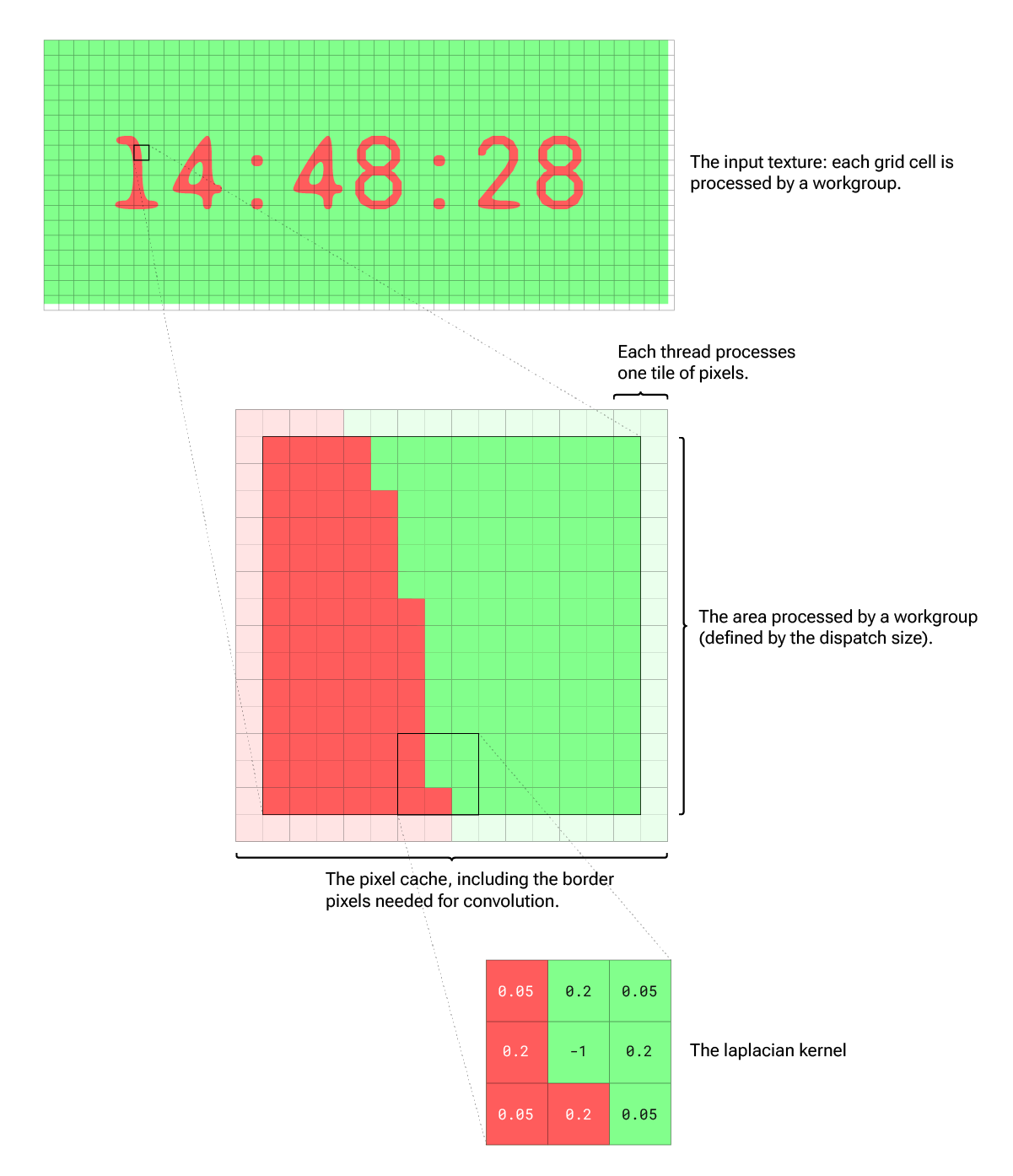
Pixels per Thread

To make every workgroup cowl a bigger space (extra pixels) we introduce a tile dimension. The tile dimension defines what number of pixels every particular person thread processes. This requires us to make use of a nested for loop inside the shader, so we’d need the preserve the tile dimension very small (e.g., 2×2).

Pixel Cache

A vital step for operating the reaction-diffusion simulation is the convolution with the laplacian kernel which is a 3×3 matrix. So, for every pixel we course of, we’ve got to learn all 9 pixels that the kernel covers with a purpose to carry out the calculation. As a result of kernel overlap from pixel to pixel, there can be a number of redundant texture reads.

Fortuitously, compute shaders permit us to share reminiscence throughout threads. So we are able to create what I name a pixel cache. The thought (from the picture blur pattern) is that every thread reads the pixels of its tile and writes them to the cache. As soon as each thread of the workgroup has saved its pixels within the cache (we guarantee this with a workgroup barrier), the precise processing solely wants to make use of the prefetched pixels from the cache. Therefore it doesn’t require any additional texture reads. The construction of the compute perform may look one thing like this:

// the pixel cache shared accross all threads of the workgroup
var<workgroup> cache: array<array<vec4f, 128>, 128>;

@compute @workgroup_size(8, 8, 1)
fn compute_main(/* ...builtin variables */ ) {

  // add the pixels of this thread's tiles to the cache
  for (var c=0u; c<2; c++) {
    for (var r=0u; r<2; r++) {
      // ... calculate the pixel coords from the builtin variables
      // retailer the pixel worth within the cache
      cache[y][x] = worth;
    }
  }

  // do not proceed till all threads have reached this level
  workgroupBarrier();

  // course of each pixel of this threads tile
  for (var c=0u; c<2; c++) {
    for (var r=0u; r<2; r++) {
        // ...carry out reaction-diffusion algorithm
        textureStore(/* ... */);
      }
    }
  }
}

However there’s one other difficult facet we’ve got to be careful for: the kernel convolution requires us to learn extra pixels than we finally course of. We may prolong the pixel cache dimension. Nevertheless, the scale of the reminiscence shared by the threads of a workgroup is restricted to 16,384 bytes. Due to this fact we’ve got to lower the dispatch dimension by (kernelSize - 1)/2 on both sides. Hopefully the next illustration will make these steps clearer.

UV Distortion

One drawback of utilizing the compute shader in comparison with the fragment shader answer is that you simply can not use a sampler for the storage textures inside a compute shader (you’ll be able to solely load integer pixel coordinates). If you wish to animate the simulation by shifting the feel area (i.e., distorting the UV coordinates in fractional increments), you must do the sampling your self.

One solution to cope with that is to make use of a handbook bilinear sampling perform. The sampling perform used within the demo relies on the one proven right here, with some changes to be used inside a compute shader. This permits us to pattern fractional pixel values:

fn texture2D_bilinear(t: texture_2d<f32>, coord: vec2f, dims: vec2u) -> vec4f {
    let f: vec2f = fract(coord);
    let pattern: vec2u = vec2u(coord + (0.5 - f));
    let tl: vec4f = textureLoad(t, clamp(pattern, vec2u(1, 1), dims), 0);
    let tr: vec4f = textureLoad(t, clamp(pattern + vec2u(1, 0), vec2u(1, 1), dims), 0);
    let bl: vec4f = textureLoad(t, clamp(pattern + vec2u(0, 1), vec2u(1, 1), dims), 0);
    let br: vec4f = textureLoad(t, clamp(pattern + vec2u(1, 1), vec2u(1, 1), dims), 0);
    let tA: vec4f = combine(tl, tr, f.x);
    let tB: vec4f = combine(bl, br, f.x);
    return combine(tA, tB, f.y);
}

That is how the pulsating motion of the simulation from the centre that may be seen within the demo was created.

Parameter Animation

One of many issues I actually like about reaction-diffusion is the number of totally different patterns you will get by altering just some parameters. If you happen to then animate these modifications over time or in response to person interplay, you will get actually fascinating results. Within the demo, for instance, some parameters change relying on the gap from the centre or the velocity of the pointer.

Composition Rendering

With the reaction-diffusion simulation accomplished, the one factor left is to attract the consequence to the display screen. That is the job of the composition render pipeline.

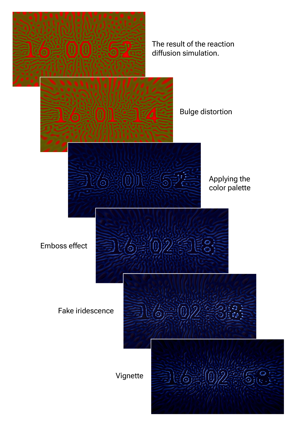
I simply wish to give a quick overview of the steps concerned within the demo software. Nevertheless, these rely very a lot on the model you wish to obtain. Listed here are the principle changes made through the composition move of the demo:

1. Bulge distortion: Earlier than sampling the reaction-diffusion consequence texture, a bulge distortion is utilized to the UV coordinates (based mostly on this shadertoy code). This provides a way of depth to the scene.
2. Color: A color palette is utilized (from Inigo Quilez)
3. Emboss filter: A easy emboss impact offers the “veins” some quantity.
4. Faux iridescence: This delicate impact relies on a unique color palette, however is utilized to the unfavorable area of the embossing consequence. The faux iridescence makes the scene appear a little bit bit extra vibrant.
5. Vignette: A vignette overlay is used to darken the sides.

Conclusion

So far as efficiency is worried, I’ve created a really primary efficiency check between a fraction variant and the compute variant (together with bilinear sampling). No less than on my machine the compute variant is lots quicker. The efficiency assessments are in a separate folder within the repository – solely a flag within the primary.js must be modified to check fragment with compute (GPU time measured with timestamp-query API).

I’m nonetheless very new to WebGPU improvement. If something in my tutorial may be improved or just isn’t right, I might be comfortable to listen to about it.

Sadly, I couldn’t go into each element and will solely clarify the thought behind utilizing a compute shader for operating a reaction-diffusion simulation very superficially. However I hope you loved this tutorial and that you simply may be capable of take a little bit one thing away with you in your personal tasks. Thanks for studying!