You’ve Obtained to be Modeling Me » Pupil Lounge

Becoming a member of us immediately is Wesley Hamilton, who’s a STEM Outreach Engineer right here at MathWorks. Wesley will discuss tackling the 2019 MathWorks Math Modeling Problem (M3C) drawback. Wesley, over to you…

Introduction

Right here we’ll deal with the 2019 M3C drawback by constructing an preliminary mannequin for the primary a part of the problem. To do that we’ll make use of greatest modeling practices, together with figuring out variables and making assumptions, in addition to use MATLAB’s information evaluation and curve becoming toolboxes to help our modeling course of. Observe that this strategy isn’t the one method groups may strategy this drawback (although a number of the high submissions did one thing related!); our objective is to see what a begin may appear to be.

M3C issues include three elements. The primary half is designed to be doable by most, if not all, groups. The following two elements sometimes construct on work from the primary half, however function extra open-ended questions that permit groups showcase their creativity and technical prowess when creating fashions and options to the said questions. As I discussed, we’ll focus in on half 1 of the 2019 M3C drawback and set ourselves up with a stable begin for tackling the remainder of the problem.

The overall define we’ll observe is

1. learn the issue in its entirety,
2. formulate a plan to reply the issue,
3. perform our plan.

Preliminary studying of the issue

We’ll begin by studying the introduction for context of the issue:

We see they supply a reference to an NPR article on Opioid overdoses in the USA. Let’s maintain off on trying on the article till we end studying the issue assertion:

Efforts, equivalent to taxes and rules on cigarettes and the Drug Abuse Resistance Schooling program, have been made on the native, state, and nationwide degree to teach, management, and/or limit the consumption of such substances. Such efforts want to start out with an understanding of how substance abuse spreads and impacts some people greater than others.

Now to half 1, what we are literally being requested to do:

Darth Vapor—Typically containing excessive doses of nicotine, vaping (inhalation of an aerosol created by vaporizing a liquid) is hooking a brand new technology that may in any other case have chosen to not use tobacco merchandise. Construct a mathematical mannequin that predicts the unfold of nicotine use as a consequence of vaping over the following 10 years. Analyze how the expansion of this new type of nicotine use compares to that of cigarettes.

The final two sentences are key, and price repeating: “Construct a mathematical mannequin that predicts the unfold of nicotine use as a consequence of vaping over the following 10 years. Analyze how the expansion of this new type of nicotine use compares to that of cigarettes.”

So, our job is to mannequin the unfold of nicotine use as a consequence of vaping and examine our mannequin to the utilization of cigarettes. Some questions I already bear in mind are: how can we measure the unfold or use? Will we hold observe of vape utilization by the variety of cartridges used? By variety of customers?

Inspecting the attachments and information

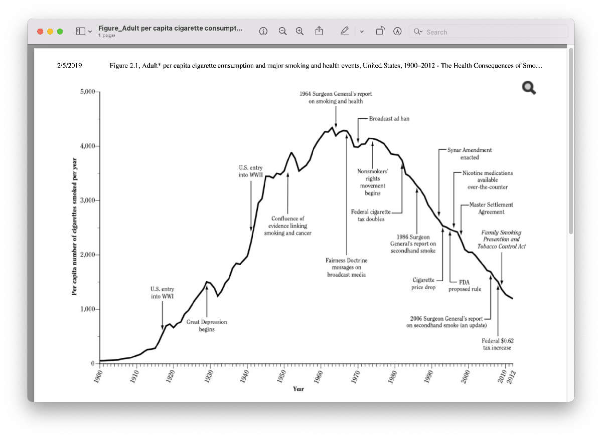
The very first thing we should always be aware of as we take a look at this graph is the labels on the axes. The x-axis has time in years, and the y-axis is labeled “per capita variety of cigarettes smoked per yr”. In case you’re undecided what per capita means, you must take a second to do a seek for that time period so you may totally perceive the which means of the information you have got. A fast search turns up that the phrase per capita is commonly used to interchange the phrases “per particular person”. So, this information provides us the typical variety of cigarettes consumed per particular person every year. This information doesn’t inform us what share of the inhabitants smokes. Nevertheless, we are able to make an assumption that if we did have that information, it’d “look” just like this information by way of form. Let’s seize that assumption in our Reside Script. If now we have time in a while, we’d seek for information to help this assumption.

Talking of form, subsequent we’d study the form of the curve. It begins close to zero on the y-axis, hits a peak within the Sixties and Seventies, after which decreases. The form of this curve jogs my memory of a Bell curve, or Regular distribution, additionally referred to as a Gaussian, from chance principle.

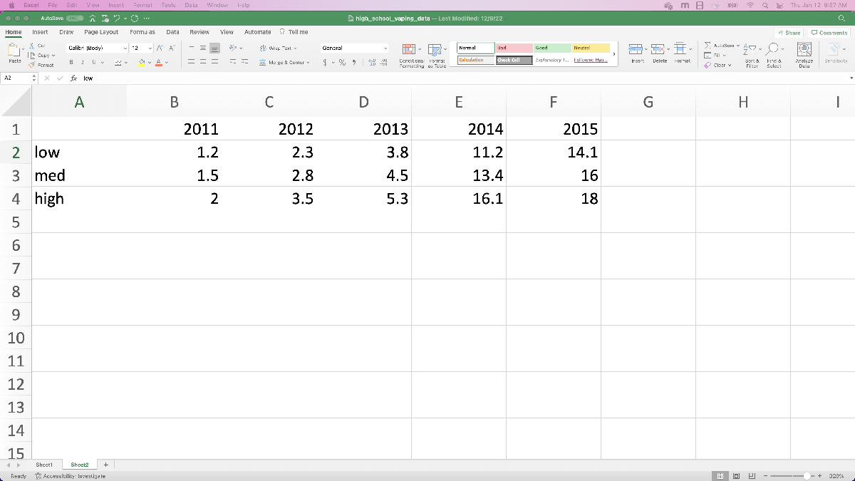
Now let’s check out the supplied information, beginning with the “high_school_vaping_data.xlsx” information. The title of the particular spreadsheet is “Proportion of Excessive Faculty College students who used e-cigarettes prior to now 30 days, by gender and race/ethnicity; Nationwide Youth Tobacco Survey, 2011-2015”.

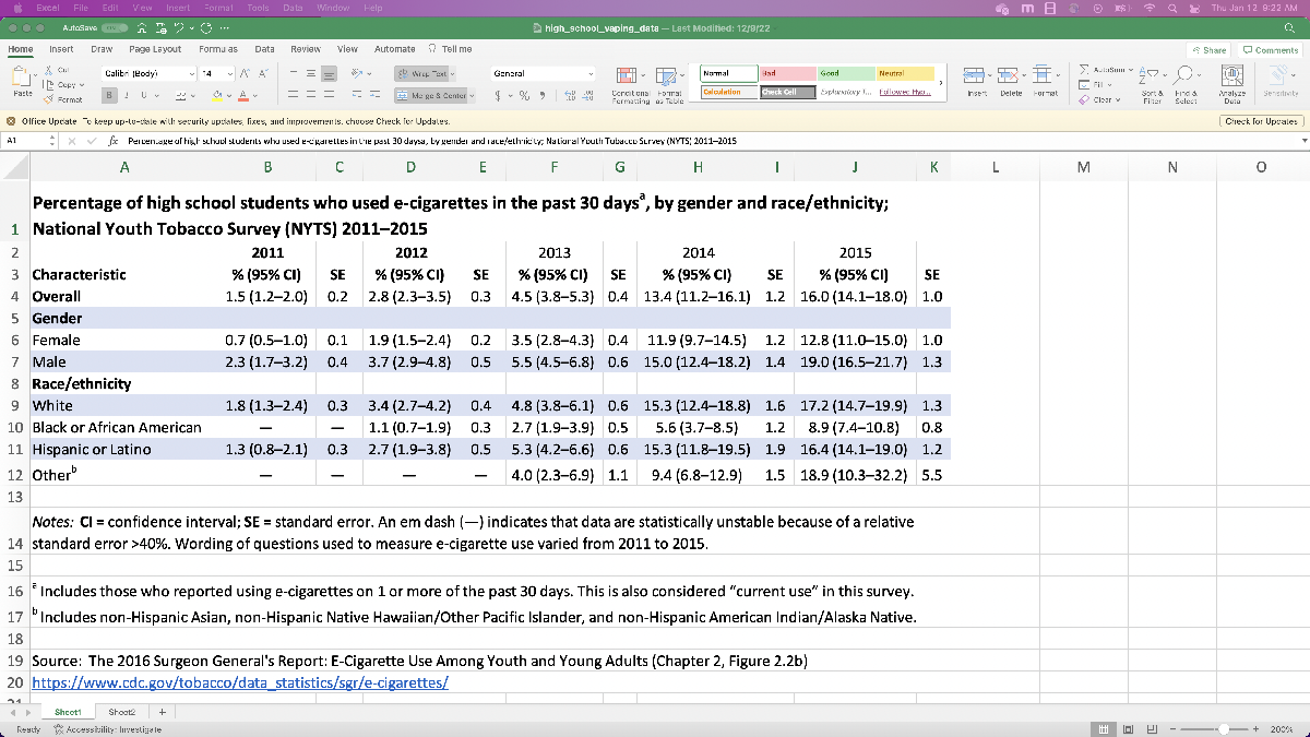
This information seems to be for all HS college students (ninth by twelfth grade), and splits it up based mostly on gender and race/ethnicity. Already it seems like we’ll have to do some pre-processing if we wish to learn within the information, as a result of it contains the share together with a confidence interval in parentheses in every cell (consider a confidence interval because the error bounds coming from the survey sampling); for MATLAB to fortunately learn it in, there needs to be a single quantity in every cell. We additionally don’t know (with out additional analysis) what share of HS college students are White or Hispanic/Latino, so we’d should put in additional work if we wish to combine and match the information objects that aren’t within the “General” row.

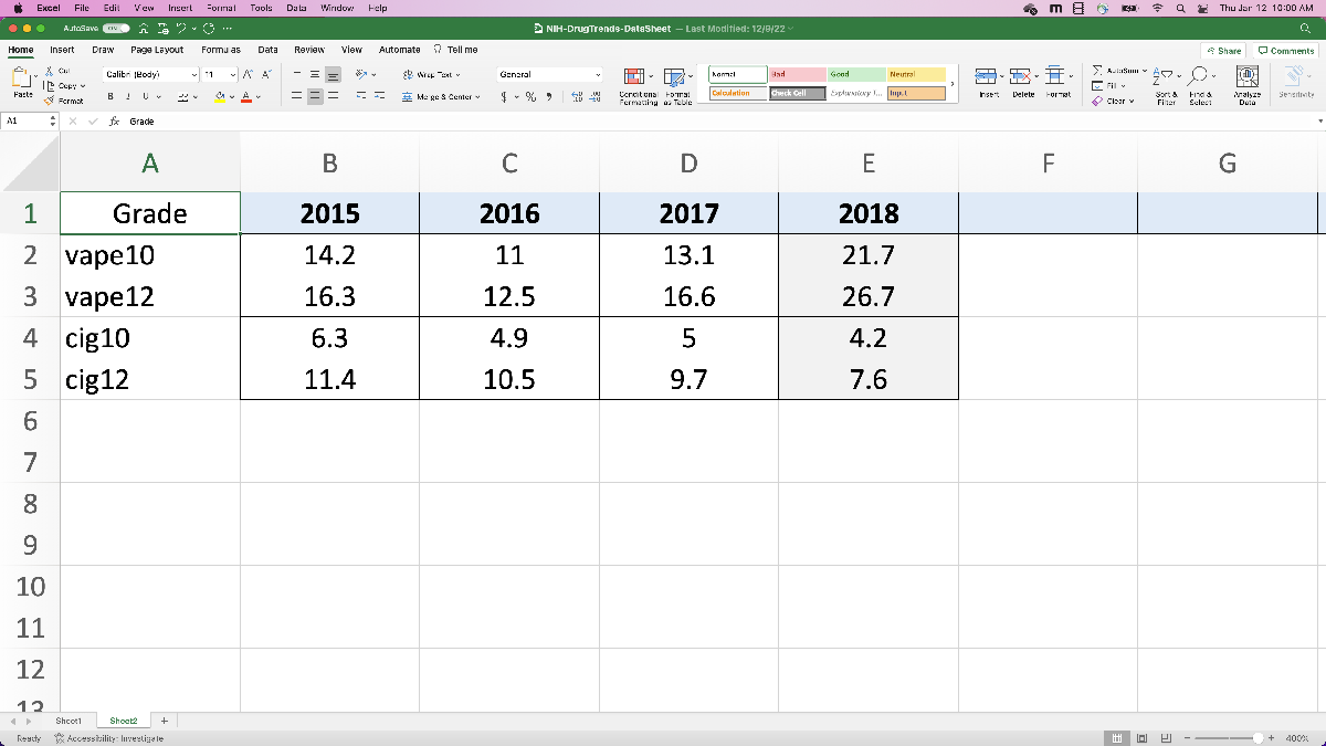
Lastly, let’s take a look at the “NIH-DrugTrends-DataSheet.xlsx”.

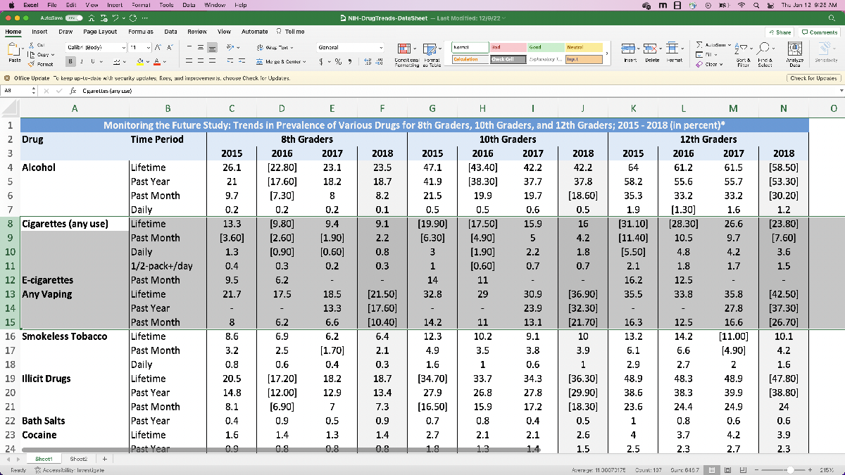
This comprises much more information on numerous medication, however particularly related for us we see the row comparable to “any vaping prior to now month”. This information is for the years 2015 to 2018, and is cut up amongst eighth grade, tenth grade, and twelfth grade. Additionally, due to how the information is formatted, we’ll should carry out just a little pre-processing earlier than we are able to learn it into MATLAB (like the opposite spreadsheet). For the reason that different information is for the years 2011 – 2015, we’d wish to merge the 2 datasets so now we have information for HS vape utilization from 2011 – 2018, which provides our mannequin extra to work with. We are able to justify this by making an assumption that “the Nationwide Youth Tobacco Survey and NIH Drug Traits information are comparable”. We’ll should resolve which dataset we use for the 2015 information, however we are able to try this after we’ve learn the information in and are beginning to construct the mannequin.

Preliminary plan for mannequin

Now that we’ve taken a take a look at the supplied information, let’s formulate an preliminary plan of assault to get began with an answer. For assumptions up to now now we have:

• cigarette per capita utilization is akin to variety of folks smoking (in order that after we go to check e-cigarette utilization with cigarette utilization, we are able to tie in that determine of historic cigarette utilization), and
• the Nationwide Youth Tobacco Survey and NIH Drug Traits information are comparable (in order that we are able to mix the 2 datasets so now we have extra information to work with).

For a plan of action, let’s:

1. Pre-process the information and browse it in.
2. Attempt to match some curves to the information to foretell utilization sooner or later. We would hope that becoming a Gaussian to the information works greatest, in order that now we have some foundation to say that e-cigarette utilization will mimic historic cigarette developments, however let’s see how the fashions behave first.
3. Write a brief abstract, which we may then copy and paste into our ultimate report.

Studying in and processing the information

Now let’s preprocess the information. For the reason that spreadsheet has the chances with confidence intervals in the identical cells, it’s best if we manually re-enter the information into a distinct sheet. It will make importing the information considerably simpler in a while. I’ve additionally integrated the arrogance intervals by together with the low (decrease sure of the interval), medium (reported survey outcome), and excessive (higher sure of the interval) estimates within the spreadsheet.

Subsequent, let’s do the identical factor with the tenth and twelfth grade information from the NIH information. Since we wish to examine vaping to cigarette utilization, let’s document each the e-cigarette and cigarette information. On this case, let’s truly use the “Any vaping” within the “previous month” information, the place we’re assuming vaping and e-cigarette utilization are comparable information. In any other case we’re going to do the identical factor as earlier than: copy the values into a brand new spreadsheet web page so that they’re simple to learn in.

To summarize the steps, we:

1. opened the “Import Information” app from the Dwelling toolbar,
2. chosen the spreadsheet “high_school_vaping_data.xlsx” which has the information we wish to import,
3. chosen Sheet 2 of the spreadsheet, and chosen the row of information we wish to begin with (because it’s just one row, let’s not hassle with importing the column labels, and since we don’t want to fret about row labels, we’ll simply import the numeric information),
4. clicked the “Import Choice” dropdown menu and chosen “Generate Script” (in order that we are able to simply modify the code later and never should undergo the app every time),
5. modified the title of the desk that’s imported into MATLAB, transformed it to an array, after which ran the code to confirm we imported the information accurately.

Since we didn’t embody a semicolon after “HSData = table2array(HSTable)”, MATLAB prints the results of that line of code, which exhibits us the contents of the array “HSData”, the information we anticipated to learn in.

Now let’s repeat the identical course of with the NIH information. Right here, we’re recording tenth and twelfth grader information for vaping and cigarette utilization. As earlier than, we choose the proper spreadsheet, go to sheet 2, choose the information (ignoring the information labels), and click on “import choice” after which “generate script”. As earlier than, let’s convert this information to an array, this time referred to as “NIHData”.

Observe that we additionally modified the view fashion for the Reside Script, in order that the output of code seems inline and to not the facet of the editor. Additionally, since we’ve copied what we wanted from the untitled.m recordsdata we are able to go forward and shut these tabs.

One level value mentioning right here: it is a comparatively small dataset, and we may have probably analyzed the information in excel instantly, and/or manually kind the information into MATLAB. The Import Information app is extremely highly effective once you begin coping with a lot bigger datasets although, particularly if you wish to hold observe of column or row labels, and is value figuring out about and getting snug with.

As soon as all of that’s achieved, we are able to get began on our mannequin! The code we generated is included right here for reference (make certain the excel spreadsheets are positioned in the identical folder as this Reside Script):

Fast Reside Script housekeeping

Now that our Reside Script is rising, let’s add in a number of part breaks and headers so it’s simpler for us to revisit and use our code. Based mostly on our technique for tackling this drawback, our sections shall be:

1. Report (the place we write our assumptions and conclusions),
2. Studying in information
3. Vape mannequin (the place we predict future vape utilization),
4. Comparability to cigarettes.

Constructing a mannequin by becoming a curve

Our plan right here shall be to mannequin vape utilization by becoming a curve to the information we’ve imported, and use the fitted curve to say one thing about future vape utilization. Two concerns come up:

• The NIH information is cut up between tenth and twelfth grade college students. How can we use this information to say one thing about highschool college students as an entire?
• We’ve got 2 datasets (the highschool vaping information and the NIH information) that cowl the years 2011 to 2015, and 2015 to 2018. Can we mix the information ultimately to have extra information factors with which to construct the mannequin?

For the primary consideration, let’s begin by averaging the tenth and twelfth grade information from the NIH for every year, and use that as an approximation for all of highschool. Implicitly we’re assuming that there are roughly the identical variety of tenth and twelfth grade college students within the research (so we are able to common the chances) and that tenth and twelfth grade college students present an affordable approximation of how all highschool college students would behave; let’s truly add this assumption to our operating record of assumptions, simply in case (we may wish to break it up into two assumptions, however we are able to resolve that later).

For the second consideration, we’re going to take the HS information from 2011 to 2014, and use the NIHdata from 2015 to 2018. Right here we’re assuming that the strategies of surveying are comparable for the 2 datasets, so it is smart to merge them. With out trying into the research themselves, one justification for this we are able to present is that the NIH information 2015 worth now we have (15.25) is throughout the confidence interval for the HS vaping information (14.1 – 18).

Our Reside Script ought to present us a plot of vape utilization per yr, as demonstrated under. Specifically, vape utilization appears to be on the rise.

As quickly as we specify the information for use, we see the information plotted with a line (1-dimensional polynomial, behind the information selector window) robotically plotted. Is a line an affordable mannequin for vape utilization? Nicely, it appears to “match” the information nicely sufficient, however what occurs as time will increase? Since we’re modeling the share of HS college students vaping, as time will increase our mannequin tells us that close to 2045, 100% of HS college students shall be vaping, close to 2050 roughly 114% of HS college students shall be vaping, and so forth. This doesn’t make sense for our drawback, and utilizing 2nd and third diploma polynomials don’t appear to do any higher: utilizing a polynomial match doesn’t look like the precise approach to go.

If we expect again to our earlier studying of the issue, the historic cigarette utilization information regarded like a Gaussian. Fortunately, Gaussians are a built-in possibility within the curve becoming app, so let’s attempt that subsequent.

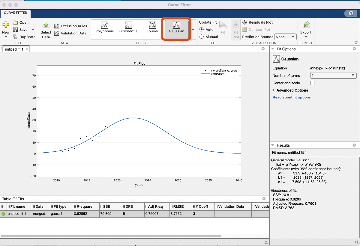
If we click on “Gaussian” within the “Match Sort” menu, our mannequin is robotically generated and appears affordable! From the plot we see that HS vape utilization will peak close to 2023 at 30%, after which have a tendency in direction of 0% utilization by round 2040. We’re proud of this for now, so let’s export the code to generate the fitted Gaussian and plot and replica it into our pocket book. To do that, we wish to click on the “Export Button” after which “Generate Code”. We are able to ignore the primary few traces and simply copy the whole lot beneath “%%Match: ‘untitled match 1’.”

Observe that this generated code additionally plots our mannequin. Let’s change a number of the settings so the plot is extra descriptive:

• Change the title to “Vape utilization prediction”,
• Plot the unique information for comparability,
• Lengthen the vary of the place we wish the fitted curve to be plotted, say 2010 to 2040 by specifying these years after which plotting that information,
• Add a legend for the unique and fitted information,
• Add a descriptive Y axis label,
• Make sure the prolonged years are displayed within the plot.

Voila, now we have our mannequin for highschool vape utilization over the following 10+ years, addressing the primary of two duties for half 1 of this problem. The mannequin in query is a Gaussian, whose equation we see on the precise within the “Curve Fitter” app: a1*exp(-((x-b1)/c1)^2), with a1 = 31.9, b1 = 2023, c1 = 7.598. In our report we’ll wish to report this mannequin, which we’ll come again to on the finish of this put up. The code we generated is included right here for reference (make certain the excel spreadsheets are positioned in the identical folder as this Reside Script):

Evaluating to historic information

The opposite job for half 1 is to check the HS cigarette utilization to the historic pattern, and the technique we’ll begin with is becoming a Gaussian to that information and evaluating to the historic pattern. This would supply additional proof that

1. the NIH information is dependable, and
2. the Gaussian is an affordable mannequin to make use of for cigarette utilization and, therefore, vape utilization.

To do that we’ll use the identical pipeline as above:

• use MATLAB’s imply perform to common the third and fourth rows of NIHdata, which have the cigarette utilization information for tenth and twelfth graders from 2015 to 2018,
• use the curve fitter app to suit a Gaussian to the information.

Step one seems identical to it did earlier than: isolate the tenth and twelfth grade cigarette utilization information and take the column-wise imply to get our HS cigarette utilization estimate.

The second step seems just like earlier than: open up the curve fitter app, specify the x and y information to make use of, and select “Gaussian” below “Match Sort”. Observe that we additionally specified a brand new vector with simply the years 2015 – 2018, since we’ll want to inform the curve fitter app which X information we wish to use and the Y information on this case isn’t your complete interval 2011-2018.

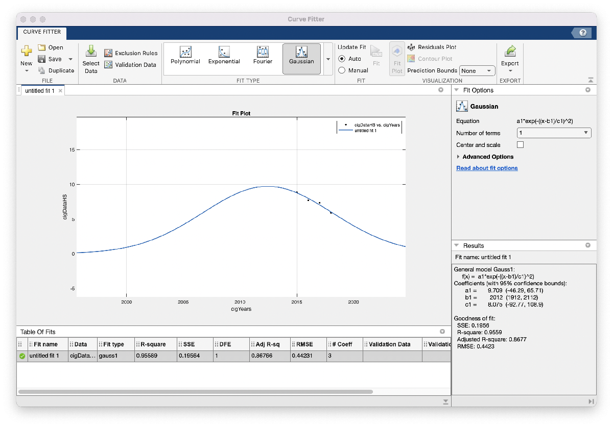
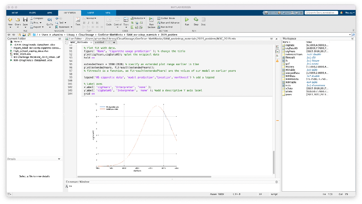
After we zoom out this time, nonetheless, the mannequin seems rather less practical: this Gaussian means that HS cigarette utilization peaked round 2012, and round 1996 was near 0 p.c utilization. We might in all probability anticipate to see the next share of HS cigarette utilization additional again in time, so possibly we gained’t embody this mannequin in our report simply but. One potential purpose for this mannequin not matching our expectations is that the quantity of information we used is comparatively small: within the vape utilization mannequin we had 8 information factors to suit our mannequin with, whereas right here we solely have 4. We’ll go forward and save the code and determine we generated so that they’re simple to return to. As we did above, we’ll change a number of the settings so the plot is extra descriptive:

• Change the title to “Vape utilization prediction”
• Plot the unique information for comparability
• Lengthen the vary of the place we wish the fitted curve to be plotted, say 1990 to 2020 by specifying these years after which plotting that information
• Add a legend for the unique and fitted information
• Add a descriptive Y axis label

We’re not prepared to incorporate this mannequin or plot in our report, however at the very least now we have the code able to go and modify if/after we discover supplementary information to enhance our mannequin. The code we generated is included right here for reference (make certain the excel spreadsheets are positioned in the identical folder as this Reside Script):

Abstract of progress and subsequent steps

One side of the competitors not but mentioned is the truth that it’s a group effort, in that (possible) it is going to be you and 1-3 of your colleagues tackling this query collectively. So, as you and your teammates proceed on within the day, one job somebody may tackle is to refine the cigarette utilization mannequin. This may imply discovering extra information factors to construct a extra correct mannequin, or attempting a distinct curve to suit the mannequin, or exploring a very totally different strategy! We may additionally revisit the mannequin we’re proud of to point out we tried different affordable fashions; polynomials didn’t appear to offer us affordable outcomes, however possibly a logistic curve or Weibull curve (no matter that’s) would give different affordable fashions.

One other job for a teammate could possibly be to revisit and add justification to the 2 assumptions we wrote down: does per capita cigarette utilization correlate with with variety of cigarette customers (possibly as a share of complete inhabitants)? can we discover information about quantity or share of cigarette customers all through historical past, possibly even HS cigarette utilization information or charts? Why are the Nationwide Youth Tobacco Survey and NIH Drug Traits datasets comparable/mergeable? And so on.

At this level we’ve more-or-less answered half 1, at the very least sufficient for us to be snug that now we have one thing we are able to write about and so we are able to get began on half 2 of the query. Earlier than studying and beginning on half 2, let’s acquire our ideas and description our resolution (up to now) to half 1:

To mannequin the unfold of nicotine utilization as a consequence of vaping over the following 10 years, we use survey information from the Nationwide Youth Tobacco Survey and NIH to suit a Gaussian mannequin on share of HS college students vaping:

share of HS college students vaping = a1*exp(-((x-b1)/c1)^2),

the place a1 = 31.9, b1 = 2023, c1 = 7.598, and x is the yr of curiosity. Our mannequin predicts vaping utilization will peak with roughly 32% of HS college students vaping by the yr 2023, afterwhich utilization will decline till almost 0% utilization by 2040. The remainder of this part describes in additional element our strategies and assumptions that help this mannequin. [Here we would include assumptions, discuss the model development including the rational for choosing a Gaussian, etc.]

We’re not achieved with half 1, however now we have a stable begin. Keep tuned for an upcoming weblog put up that examines some scholar submissions to this problem, and a number of the fashions their groups constructed!