

I’ve seen stuff you folks would not imagine.
Valleys sculpted by trigonometric capabilities.
Charges on fireplace off the shoulder of divergence.
Beams glitter in the dead of night close to the Polyak gate.
All these landscapes can be misplaced in time, like tears in rain.
Time to halt.A momentum optimizer *
$$
defaa{boldsymbol a}
defrr{boldsymbol r}
defAA{boldsymbol A}
defHH{boldsymbol H}
defEE{mathbb E}
defII{boldsymbol I}
defCC{boldsymbol C}
defDD{boldsymbol D}
defKK{boldsymbol Ok}
defeeps{boldsymbol varepsilon}
deftr{textual content{tr}}
defLLambda{boldsymbol Lambda}
defbb{boldsymbol b}
defcc{boldsymbol c}
defxx{boldsymbol x}
defzz{boldsymbol z}
defuu{boldsymbol u}
defvv{boldsymbol v}
defqq{boldsymbol q}
defyy{boldsymbol y}
defss{boldsymbol s}
defpp{boldsymbol p}
deflmax{L}
deflmin{mu}
defRR{mathbb{R}}
defTT{boldsymbol T}
defQQ{boldsymbol Q}
defCC{boldsymbol C}
defEcond{boldsymbol E}
DeclareMathOperator*{argmin}{{arg,min}}
DeclareMathOperator*{argmax}{{arg,max}}
DeclareMathOperator*{reduce}{{reduce}}
DeclareMathOperator*{dom}{mathbf{dom}}
DeclareMathOperator*{Repair}{mathbf{Repair}}
DeclareMathOperator{prox}{mathbf{prox}}
DeclareMathOperator{span}{mathbf{span}}
DeclareMathOperator{Ima}{Im}
defdefas{stackrel{textual content{def}}{=}}
defdif{mathop{}!mathrm{d}}
definecolor{colormomentum}{RGB}{27, 158, 119}
definecolor{colorstepsize}{RGB}{217, 95, 2}
defmom{{colour{colormomentum}m}}
defstep{{colour{colorstepsize}h}}
$$
Gradient Descent with Momentum
Gradient descent with momentum,
designed to unravel unconstrained minimization issues of the shape
start{equation}
argmin_{xx in RR^d} f(xx),,
finish{equation}
the place the target perform $f$ is differentiable and we now have entry to its gradient $nabla
f$. On this methodology
the replace is a sum of two phrases. The primary time period is the
distinction between the present and the earlier iterate $(xx_{t} – xx_{t-1})$, also referred to as momentum
time period. The second time period is the gradient $nabla f(xx_t)$ of the target perform.
Gradient Descent with Momentum
Enter: beginning guess $xx_0$, step-size $step > 0$ and momentum
parameter $mother in (0, 1)$.
$xx_1 = xx_0 – dfrac{step}{mother+1} nabla f(xx_0)$
For $t=1, 2, ldots$ compute
start{equation}label{eq:momentum_update}
xx_{t+1} = xx_t + mother(xx_{t} – xx_{t-1}) – stepnabla
f(xx_t)
finish{equation}
Regardless of its simplicity, gradient descent with momentum reveals unexpectedly wealthy dynamics that we’ll discover on this publish.
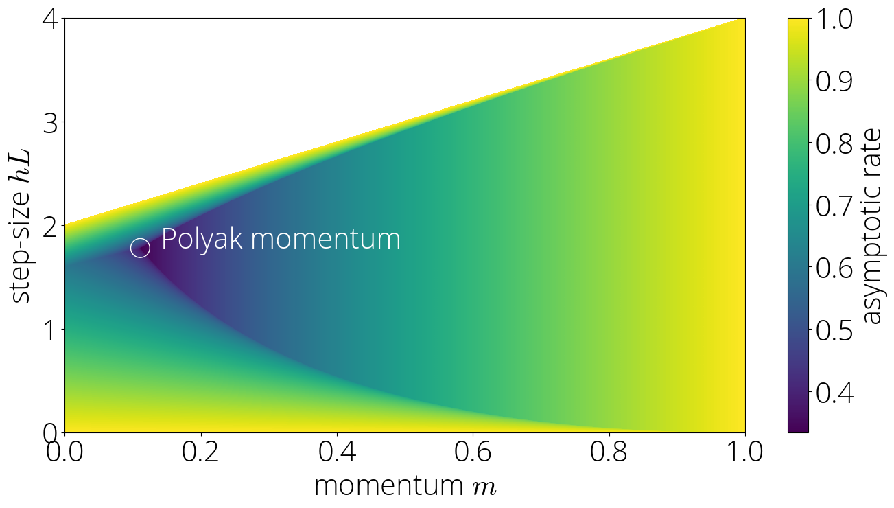
The panorama described within the part “The Dynamics of Momentum” are completely different than those described on this publish. Those in Gabriel’s paper describe the advance alongside the course of a single eigenvector, and as such are at greatest a partial view of convergence (actually, they provide the deceptive impression that one of the best convergence is achieved with zero momentum). The methods used on this publish permit as an alternative to compute the worldwide convergence fee, and figures just like the above appropriately predict a non-trivial optimum momentum time period.
Convergence charges
Within the final publish we noticed that, assuming $f$ is a quadratic goal of the shape
start{equation}label{eq:choose}
f(xx) defas frac{1}{2}xx^prime HH xx + bb^prime xx~,
finish{equation}
then we will analyze gradient descent with momentum utilizing a convex mixture of Chebyshev polynomials of the primary and second form.
Extra exactly, we confirmed that the error at iteration $t$ could be bounded as
start{equation}label{eq:theorem}
|xx_t – xx^star| leq underbrace{max_{lambda in [lmin, L]} |P_t(lambda)|}_{defas r_t} |xx_0 – xx^star|,.
finish{equation}
the place $lmin$ and $L$ are the smallest and largest eigenvalues of $HH$ respectively and $P_t$ is a $t$-th diploma polynomial that we will write as
start{align}
P_t(lambda) = mother^{t/2} left( {smallfrac{2mom}{1+mother}}, T_t(sigma(lambda)) + {smallfrac{1 – mother}{1 + mother}},U_t(sigma(lambda))proper),.
finish{align}
the place $sigma(lambda) = {smalldfrac{1}{2sqrt{mother}}}(1 +
mother –
step,lambda),$ is a linear perform that we’ll seek advice from because the hyperlink perform and $T_t$ and $U_t$ are the Chebyshev polynomials of the primary and second form respectively.
We’ll denote by $r_t$ the utmost of this polynomial over the $[lmin, L]$ interval, and name the convergence fee of an algorithm the $t$-th root of this amount, $sqrt[t]{r_t}$. We’ll additionally use usually the restrict superior of this amount, $limsup_{t to infty} sqrt[t]{r_t}$, which we’ll name the asymptotic fee. The asymptotic fee supplies a handy method to examine the (asymptotic) pace of convergence, because it permits to disregard different slower phrases which might be negligible for big $t$.
This id between gradient descent with momentum and Chebyshev polynomials opens the door to deriving the asymptotic properties of the optimizer from these of Chebyshev polynomials.
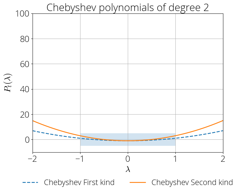
The Two Faces of Chebyshev Polynomials
Chebyshev polynomials behave very in a different way inside and out of doors the interval $[-1, 1]$. Inside this interval (shaded blue area) the magnitude of those polynomials stays near zero, whereas exterior it explodes:
![]()
Let’s make this statement extra exact.
Inside the $[-1, 1]$ interval, Chebyshev polynomials admit the trigonometric definitions $T_t(cos(theta)) = cos(t theta)$ and $U_{t}(cos(theta)) = sin((t+1)theta) / sin(theta)$ and they also have an oscillatory conduct with values bounded in absolute worth by 1 and $t+1$ respectively.
Exterior of this interval the Chebyshev polynomials of the primary form admit the specific type for $|xi| ge 1$:
start{align}
T_t(xi) &= dfrac{1}{2} Huge(xi-sqrt{xi^2-1} Huge)^t + dfrac{1}{2} Huge(xi+sqrt{xi^2-1} Huge)^t
U_t(xi) &= frac{(xi + sqrt{xi^2 – 1})^{t+1} – (xi – sqrt{xi^2 – 1})^{t+1}}{2 sqrt{xi^2 – 1}},.
finish{align}
We’re occupied with convergence charges, so we’ll look into $t$-th root asymptotics of the portions.
start{equation}
lim_{t to infty} sqrt[t]T_t(xi) = lim_{t to infty} sqrt[t] = |xi| + sqrt{xi^2 – 1},.
finish{equation}
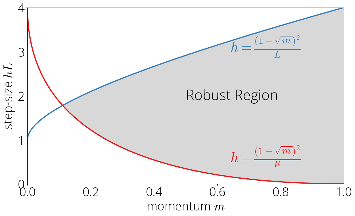
The Strong Area
Let’s begin first by contemplating the case wherein the Chebyshev polynomials are solely evaluated within the $[-1, 1]$. Because the Chebsyshev polynomials are evaluated at $sigma(cdot)$, this suggests that $|sigma(lambda)| leq 1$. We’ll name the set of step-size and momentum parameters for which the earlier inequality is verified the sturdy area.
Let’s visualize this area in a map.
Since $sigma$ is a linear perform, its extremal values are reached on the edges:
start{equation}
max_{lambda in [lmin, L]} |sigma(lambda)| = max, ,.
finish{equation}
Utilizing $lmin leq L$ and that $sigma(lambda)$ is lowering in $lambda$, we will simplify the situation that the above is smaller than one to $sigma(lmin) leq 1$ and $sigma(L) geq -1$, which by way of the step-size and momentum correspond to:
start{equation}label{eq:robust_region}
frac{(1 – sqrt{mother})^2}{lmin} leq step leq frac{(1 + sqrt{mother})^2}{L} ,.
finish{equation}
These two situations present the higher and decrease certain of the sturdy area.
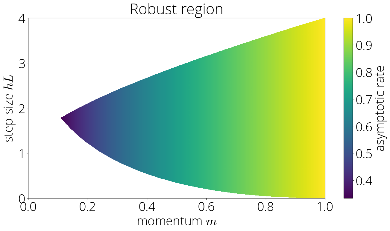
Asymptotic fee
Let $sigma(lambda) = cos(theta)$ for some $theta$, which is all the time doable since $sigma(lambda) in [-1, 1]$. On this regime, Chebyshev polynomials confirm the identities $T_t(cos(theta)) = cos(t theta)$ and $U_t(cos(theta)) = sin((t+1)theta)/sin(theta)$ , which changing within the definition of the residual polynomial offers
start{equation}
P_t(sigma^{-1}(cos(theta))) = mother^{t/2} left[ {smallfrac{2mom}{1+mom}}, cos(ttheta) + {smallfrac{1 – mom}{1 + mom}},frac{sin((t+1)theta)}{sin(theta)}right],.
finish{equation}
Because the expression contained in the sq. brackets is bounded in absolute worth by $t+2$, taking $t$-th root after which limits we now have $limsup_{t to infty} sqrt[t]{|P_t(sigma^{-1}(cos(theta)))|} = sqrt{mother}$ for any $theta$. This offers our first asymptotic fee:
The asymptotic fee within the sturdy area is $sqrt{mother}$.
That is nothing in need of magical. It will appear pure –and this would be the case in different areas– that the pace of convergence ought to rely upon each the step-size and the momentum parameter. But, this outcome implies that it isn’t the case within the sturdy area. On this area, the convergence solely is determined by the momentum parameter $mother$. Wonderful.
insensitivity to step-size has been leveraged by Zhang et al. 2018 to develop a momentum tuner
This additionally illustrates why we name this the sturdy area. In its inside, perturbing the step-size in a approach that we keep inside the area has no impact on the convergence fee. The following determine shows the asymptotic fee (darker is quicker) within the sturdy area.
![]()
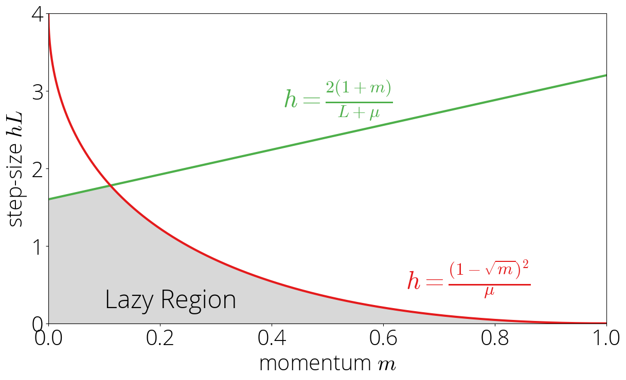
The Lazy Area
Let’s contemplate now what occurs exterior of the sturdy area. On this case, the convergence will rely upon the biggest of $, $. We’ll contemplate first the case wherein the utmost is $|sigma(lmin)|$ and go away the opposite one for subsequent part.
This area is set by the inequalities $|sigma(lmin)| > 1$ and $|sigma(lmin)| geq |sigma(L)|$.
Utilizing the definition of $sigma$ and fixing for $step$ offers the equal situations
start{equation}
step leq frac{2(1 + mother)}{L + lmin} quad textual content{ and }quad step leq frac{(1 – sqrt{mother})^2}{lmin},.
finish{equation}
Word the second inequality is identical one as for the sturdy area eqref{eq:robust_region} however with the inequality signal reversed, and so the area can be on the oposite facet of that curve. We’ll name this the lazy area, as in growing the momentum will take us out of it and into the sturdy area.
The lazy area depicted in grey within the left: decrease bounded by zero and higher bounded by the minimal of $h = frac{(1 – sqrt{m})^2}{lmin}$ and $h = frac{2(1 + m)}{L – lmin}$.
![]()
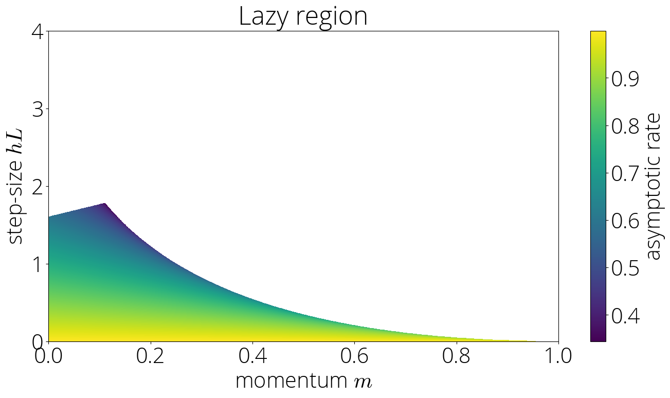
Asymptotic fee
As we noticed in Part 2, exterior of the $[-1, 1]$ interval each Chebyshev have easy $t$-th root asymptotics.
Utilizing this and that each sorts of Chebyshev polynomials agree in signal exterior of the $[-1, 1]$ interval we will compute the asymptotic fee as
start{align}
lim_{t to infty} sqrt[t]{r_t} &= sqrt{mother} lim_{t to infty} sqrt[t]{ {smallfrac{2mom}{mother+1}}, T_t(sigma(lmin)) + {smallfrac{1 – mother}{1 + mother}},U_t(sigma(lmin))}
&= sqrt{mother}left(|sigma(lmin)| + sqrt{sigma(lmin)^2 – 1} proper)
finish{align}
This offers the asymptotic fee for this area
Within the lazy area the asymptotic fee is $sqrt{mother}left(|sigma(lmin)| + sqrt{sigma(lmin)^2 – 1} proper)$.
Not like within the sturdy area, this fee is determined by each the step-size and the momentum parameter, which enters within the fee by way of the hyperlink perform $sigma$. This may be noticed within the colour plot of the asymptotic fee
![]()
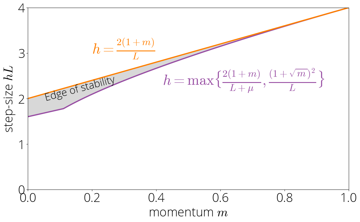
Knife’s edge
The sturdy and lazy area occupy most (however not all!) of the area for which momentum converges. There is a small area that sits between the lazy and sturdy areas and the area the place momentum diverges. We name this area the Knife’s edge
For parameters not within the sturdy or lazy area, we now have that $|sigma(L)| > 1$ and $|sigma(L)| > |sigma(lmin)|$. Utilizing the asymptotics of Chebyshev polynomials as we did within the earlier part, we now have that the asymptotic fee is $sqrt{mother}left(|sigma(L)| + sqrt{sigma(L)^2 – 1} proper)$. The tactic will solely converge when this asymptotic fee is under 1. Implementing this ends in $step lt 2 (1 + mother) / L$. Combining this situation with the considered one of not being within the sturdy or lazy area offers the characterization:
start{equation}
step lt frac{2 (1 + mother)}{L} quad textual content{ and } quad step geq maxBig{tfrac{2(1 + mother)}{L + lmin}, tfrac{(1 + sqrt{mother})^2}{L}Huge},.
finish{equation}
![]()
Asymptotic fee
The asymptotic fee could be computed utilizing the identical approach as within the lazy area. The ensuing fee is identical as in that area however with $sigma(L)$ changing $sigma(lmin)$:
Within the Knife’s edge area the asymptotic fee is $sqrt{mother}left(|sigma(L)| + sqrt{sigma(L)^2 – 1} proper)$.
Pictorially, this corresponds to
![]()

Placing all of it collectively
That is the top of our journey. We have visited all of the areas on which momentum converges.
The asymptotic fee $limsup_{t to infty} sqrt[t]{r_t}$ of momentum is
start{alignat}{2}
&sqrt{mother} &&textual content{ if }step in large[frac{(1 – sqrt{mom})^2}{lmin}, frac{(1+sqrt{mom})^2}{L}big]
&sqrt{mother}(|sigma(lmin)| + sqrt{sigma(lmin)^2 – 1}) &&textual content{ if } step in large[0, min{tfrac{2(1 + mom)}{L + lmin}, tfrac{(1 – sqrt{mom})^2}{lmin}}big]
&sqrt{mother}(|sigma(L)| + sqrt{sigma(L)^2 – 1})&&textual content{ if } step in large[maxbig{tfrac{2(1 + mom)}{L + lmin}, tfrac{(1 + sqrt{mom})^2}{L}big}, tfrac{2 (1 + mom) }{L} big)
&geq 1 text{ (divergence)} && text{ otherwise.}
end{alignat}
Plotting the asymptotic rates for all regions we can see that Polyak momentum (the method with momentum $mom = left(frac{sqrt{L} – sqrt{lmin}}{sqrt{L} + sqrt{lmin}}right)^2$ and step-size $step = left(frac{2}{sqrt{L} + sqrt{lmin}}right)^2$ which is asymptotically optimal among the momentum methods with constant coefficients) is at the intersection of the three regions.
![]()
Citing
If you find this blog post useful, please consider citing it as:
A Hitchhiker’s Guide to Momentum., Fabian Pedregosa, 2021
Bibtex entry:
    @misc{pedregosa2021residual,
      title={A Hitchhiker's Guide to Momentum},
      author={Pedregosa, Fabian},
      url = {http://fa.bianp.net/blog/2021/hitchhiker/},
      year={2021}
    }
Acknowledgements.
Thanks to Baptiste Goujaud for proofreading, catching many typos and making excellent clarifying suggestions, to Robert Gower for proofreading this post and providing thoughtful feedback. Thanks also to Courtney Paquette and Adrien Taylor for reporting errors.