

We’ve been investigating a latest bug report about fitnlm, the Statistics and Machine Studying Toolbox operate for strong becoming of nonlinear fashions.
Contents
Quahogs
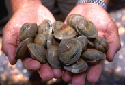
The bug report comes from Greg Pelletier, an impartial analysis scientist and biogeochemical modeler in Olympia, Washington. Greg has been learning the vulnerability of delicate marine organisms to will increase in ocean acidification. Some of the necessary of those organisms is Mercenaria mercenaria, the arduous clam.
Particularly right here in New England, arduous clams are identified by their conventional Native American identify, quahog. They’ve a well-deserved popularity for making wonderful clam chowder.
Acidification
We’re all conscious of accelerating ranges of carbon dioxide within the earth’s environment. We will not be as conscious of the impact this improve has on the well being of the earth’s oceans. Based on NOAA, the ocean absorbs about 30% of the atmospheric carbon dioxide.
A definitive and controversial 2009 paper by Justin Ries and colleagues, then on the Woods Gap Oceanographic Establishment, is “Marine calcifiers exhibit combined responses to CO2-induced ocean acidification”, https://doi.org/10.1130/G30210A.1. The arduous clam instance in Greg’s bug report comes from determine 1K within the Ries et al. paper.
The impartial variable in experiments is the ratio of alkalinity of sea water to the focus of dissolved inorganic carbon. The dependent variable is the calcification price, which compares how briskly the organism builds its shells to how briskly the shells are dissolving.

Separable Least Squares
The mannequin chosen by Ries at al. is
$$ y approx beta_1 + beta_2 e^{lambda t} $$
the place $t$ is the ratio of alkalinity to dissolved carbon and $y$ is the calcification price. The information have solely 4 distinct values of $t$, with a number of observations of $y$ at every worth.
The parameters $beta_1$, $beta_2$ and $lambda$ are decided by least squares curve match. This can be a separable least squares downside. For any given worth of $lambda$, the parameters $beta_1$ and $beta_2$ happen linearly and the least squares resolution might be obtained by MATLAB’s backslash.
Gene Golub and Victor Pereyra described separable least squares in 1973 and proposed fixing it by a variable projection algorithm. Since 1973 plenty of folks, together with Pereyra, Linda Kaufman, Fred Krogh, John Bolstadt and David Homosexual, have contributed to the event of a collection of Fortran applications named varpro. In 2011, Dianne O’Leary and Burt Rust created a MATLAB model of varpro. Their report, https://www.cs.umd.edu/~oleary/software program/varpro/, is an effective background supply, in addition to documentation for varpro.m.
I’ve a bit on separable least squares, and an instance, expfitdemo, in NCM, Numerical Computing with MATLAB. I’ve modified expfitdemo to work on Greg’s quahogs downside.
Centering Information
It seems that the issue Greg encountered might be traced to the truth that the information are usually not centered. The given values of $t$ are all constructive. This causes fitnlm to print a warning message and try and rectify the scenario by altering the levels of freedom from 22 to 23, however this solely makes the scenario worse. (We must always take one other have a look at the portion of fitnlm that adjusts the levels of freedom.)
It’s all the time a good suggestion in curve becoming to middle the information with one thing like
t = t - imply(t)
The values of $y$ are already fairly effectively centered. Rescaling $y$ with
y = 10000*y
makes interpretation of outcomes simpler.
Exponential Becoming
With the information centered and scaled, we’ve got three other ways of tackling Greg’s downside. All three strategies agree on the outcomes they compute.
- fitnlm. Treats all parameters as in the event that they had been nonlinear. Computes statistical portions resembling R-squared and RMS Error.
- varpro. Venerable software program historical past. Just one nonlinear parameter for the quahogs downside. Delivers extra statistical portions in Regression construction.
- quahogsfit. Textbook separable least squares code. Modification for the quahogs downside of expfitdemo from NCM. Just one nonlinear parameter. No statistics.
Outcomes
Nonlinear regression mannequin:
    y ~ param1 + param2*exp(param3*xval)
Estimated Coefficients:
              Estimate      SE        tStat       pValue
              ________    _______    _______    __________
    param1     0.69536     0.1657     4.1964    0.00037344
    param2    -0.26482    0.19909    -1.3302       0.19709
    param3     -22.218     8.1494    -2.7263      0.012327
Variety of observations: 25, Error levels of freedom: 22
Root Imply Squared Error: 0.307
R-Squared: 0.828,  Adjusted R-Squared 0.813
F-statistic vs. fixed mannequin: 53, p-value = 3.86e-09
Linear Parameters:
  0.695367   -0.264837
Nonlinear Parameters:
 -22.217495
Norm         of weighted residual  =   1.438935
Norm         of knowledge vector        =   3.545820
Anticipated error of observations     =   0.306782
Coefficient of willpower       =   0.828145
Regression.t_ratio
    4.1962
   -1.3301
   -2.7264
Regression.std_param
    0.1657
    0.1991
    8.1490
lambda =
  -22.2180
condX =
    4.3882
beta =
    0.6954
   -0.2648
normres =
    1.4389
quahogsfit produces this plot, which might be in contrast with determine 1K from Ries et al, reproduced above.

Software program
The codes for this submit can be found right here quahogs_driver.m and right here varpro.m.
Thanks
Due to Greg Pelletier for the bug report and to Tom Lane for his statistical experience.
Revealed with MATLAB® R2023a