ARLS, Robotically Regularized Least Squares » Cleve’s Nook: Cleve Moler on Arithmetic and Computing

(I’ve a visitor blogger at this time. Ron Jones labored with me in 1985 for his Ph. D. from the College of New Mexico. He retired lately after practically 40 years at Sandia Nationwide Labs in Albuquerque and now has an opportunity to return to the issue he studied in his thesis. — CBM)

by Rondall Jones, rejones7@msn.com

Our curiosity is in mechanically fixing troublesome linear techniques,

  A*x = b

Such techniques typically come up, for instance, in “inverse issues” by which the analyst is making an attempt to reverse the results of pure smoothing processes equivalent to warmth dissipation, optical blurring, or oblique sensing. These issues exhibit “ill-conditioning”, which implies that the answer outcomes are overly delicate to insignificant adjustments to the observations, that are given within the right-hand-side vector, b .

Here’s a graphic exhibiting this conduct utilizing a typical take a look at matrix, a 31 x 31 Hilbert matrix, with the blue line being the perfect resolution that one would hope a solver might compute. The jagged crimson line exhibits the results of a standard solver on this downside.

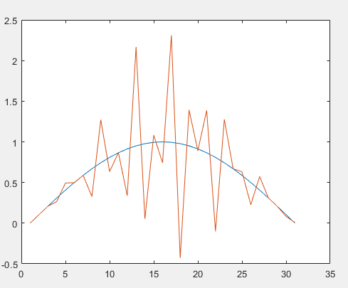
In truth this graph is extraordinarily delicate: the magnitude of the oscillations typically measure within the thousands and thousands, not just a bit bigger than the true resolution. Historically analysts have approached this problem within the linear algebraic system context by appending equations to A*x = b that request every resolution worth, x(i), to be zero. Then, one weights these conditioning equations utilizing a parameter often known as “lambda”. We’ll name it p right here. What we’ve to unravel then is that this expanded linear system:

   [ A ; p*I] * x = [b; 0]

If we decompose A into its Singular Worth Decomposition

   A = U * S * V'

and multiply each side by the transpose of the augmented LHS, the ensuing resolution to is

   x = V * inv(S^2 + p^2*I) * S * U' * b

as an alternative of the same old

   x = V * inv(S) * U' * b

It’s handy within the following dialogue to signify this as

   x = V * PCV

the place

   PCV = inv(S) * U' * b

is what we name the Picard Situation Vector. Then x is computed within the standard SVD method with the change that every singular worth S(i) is changed by

   S(i) + p^2/S(i)

This course of is known as Tikhonov regularization.

Utilizing Tikhonov regularization efficiently requires in some way selecting an applicable worth for p. Cleve Moler has for a few years jokingly used the time period “eyeball norm” to explain tips on how to decide p. “Strive numerous values of p and decide the ensuing resolution (or its graph) that ‘seems good'”.

My early work in trying to find out lambda mechanically was based mostly as an alternative on figuring out when the PCV begins to noticeably diverge. Past that time one may be pretty positive that noise in b is inflicting U'*b to lower extra slowly than inv(S) is growing, so their product, which is the PCV, begins rising unacceptably. Such an algorithm may be made to work and variations of my work have been obtainable in numerous types through the years. However figuring out the place the PCV begins rising unacceptably (which I seek advice from because the usable rank) is predicated on heuristics, transferring averages, and such, as of which require decisions of transferring common lengths and different such parameters. This isn’t an optimum state of affairs, so a I started making an attempt to revamp algorithms that don’t use any heuristics.

How can we do this algorithmically? Per Christian Hansen gave a clue to this query when he mentioned (my re-phrasing) that “the analyst mustn’t anticipate a great resolution for such an issue except the PCV is ‘declining'”. We be aware that this adage is a context-specific utility of a common requirement that when a perform is represented by an orthogonal enlargement the coefficients of the orthogonal foundation capabilities ought to finally decline towards zero. If this conduct doesn’t occur, then usually both the mannequin is incomplete or the info is contaminated. In our case the orthogonal foundation is just the columns of V, and b is the set of coefficients that will be anticipated to say no. An excellent working definition of “declining” has been arduous to nail down. The algorithm in ARLS has carried out this idea utilizing two particular important steps:

So, Section 1 of ARLS searches a wide range of values of p (keep in mind, p is Tikhonov’s “lambda”) to discover a worth simply barely massive sufficient to make the slope of the parabolic match totally damaging or zero. This offers us a decent decrease certain for the “appropriate” worth of p.

Section 2 of ARLS is way easier. Since p is the minimal usable regularization parameter, the answer tends to be much less easy and fewer near the perfect resolution than optimum. So we merely improve p barely to let the form of the graph of x easy out. Our present implementation will increase p till the residual (that’s, norm(A*x-b)) of the answer will increase by an element of two. That is, sadly, a heuristic. However an applicable worth of it may be decided by “tuning” the algorithm on a variety of take a look at issues.

We name this new algorithm Logarithmic Picard Situation Evaluation. (If the issues you’re employed on appear to wish a bit extra rest you may, in fact, improve the quantity 2 a bit. It’s 5 traces from the underside of the file.) Within the instance proven within the graphic above, ARLS produces the blue line so intently that the perfect resolution and ARLS computed resolution are indistinguishable.

Along with ARLS(A,b) itself, we offer two constrained solvers constructed on ARLS that are known as identical to ARLS:

Strive ARLS. It is obtainable from the MATLAB Central File Trade, #130259, at this hyperlink.

Get the MATLAB code

Revealed with MATLAB® R2023a