


How-To’s


How do you determine uncommon patterns in information which may reveal essential points or hidden alternatives? Anomaly detection helps determine information that deviates considerably from the norm. Time sequence information, which consists of knowledge collected over time, usually consists of tendencies and seasonal patterns. Anomalies in time sequence information happen when these patterns are disrupted, making anomaly detection a invaluable software in industries like gross sales, finance, manufacturing, and healthcare.
As time sequence information has distinctive traits like seasonality and tendencies, specialised strategies are required to detect anomalies successfully. On this weblog put up, we’ll discover some well-liked strategies for anomaly detection in time sequence, together with STL decomposition and LSTM prediction, with detailed code examples that can assist you get began.
Time sequence anomaly detection in companies
Time sequence information is important to many companies and providers. Many companies document information over time with timestamps, permitting adjustments to be analyzed and information to be in contrast over time. Time sequence are helpful when evaluating a sure amount over a sure interval, as, for instance, in a year-over-year comparability the place the information displays traits of seasonalities.
Gross sales monitoring
One of the widespread examples of time sequence information with seasonalities is gross sales information. As plenty of gross sales are affected by annual holidays and the time of the 12 months, it’s arduous to attract conclusions about gross sales information with out contemplating the seasonalities. Due to that, a typical methodology for analyzing and discovering anomalies in gross sales information is STL decomposition, which we’ll cowl intimately later on this weblog put up.
Finance
Monetary information, comparable to transactions and inventory costs, are typical examples of time sequence information. Within the finance trade, analyzing and detecting anomalies on this information is a typical follow. For instance, time sequence prediction fashions can be utilized in computerized buying and selling. We’ll use a time sequence prediction to determine anomalies in inventory information later on this weblog put up.
Manufacturing
One other use case of time sequence anomaly detection is monitoring defects in manufacturing strains. Machines are sometimes screens, making time sequence information accessible. Having the ability to notify administration of potential failures is important, and anomaly detection performs a key function.
Medication and healthcare
In medication and healthcare, human vitals are monitored and anomalies could be detected. That is essential sufficient in medical analysis, however it’s essential in diagnostics. If a affected person at a hospital has anomalies of their vitals and isn’t handled instantly, the outcomes could be deadly.
Why is it essential to make use of particular strategies for time sequence anomaly detection?
Time sequence information is particular within the sense that it generally can’t be handled like different kinds of information. For instance, after we apply a practice check break up to time sequence information, the sequentially associated nature of the information means we can’t shuffle it. That is additionally true when making use of time sequence information to a deep studying mannequin. A recurrent neural community (RNN) is usually used to take the sequential relationship into consideration, and coaching information is enter as time home windows, which protect the sequence of occasions inside.
Time sequence information can also be particular as a result of it usually has seasonality and tendencies that we can’t ignore. This seasonality can manifest in a 24-hour cycle, a 7-day cycle, or a 12-month cycle, simply to call just a few widespread prospects. Anomalies can solely be decided after the seasonality and tendencies have been thought of, as you will note in our instance under.
Strategies used for anomaly detection in time sequence
As a result of time sequence information is particular, there are particular strategies for detecting anomalies in it. Relying on the kind of information, a number of the strategies and algorithms we talked about within the earlier weblog put up about anomaly detection can be utilized on time sequence information. Nevertheless, with these strategies, the anomaly detection is probably not as strong as utilizing ones particularly designed for time sequence information. In some instances, a mixture of detection strategies can be utilized to reconfirm the detection consequence and keep away from false positives or negatives.
STL decomposition
One of the well-liked methods to make use of time sequence information that has seasonality is STL decomposition – seasonal development decomposition utilizing LOESS (domestically estimated scatterplot smoothing). On this methodology, a time sequence is decomposed utilizing an estimate of seasonality (with the interval supplied or decided utilizing an algorithm), a development (estimated), and the residual (the noise within the information). A Python library that gives STL decomposition instruments is the statsmodels library.
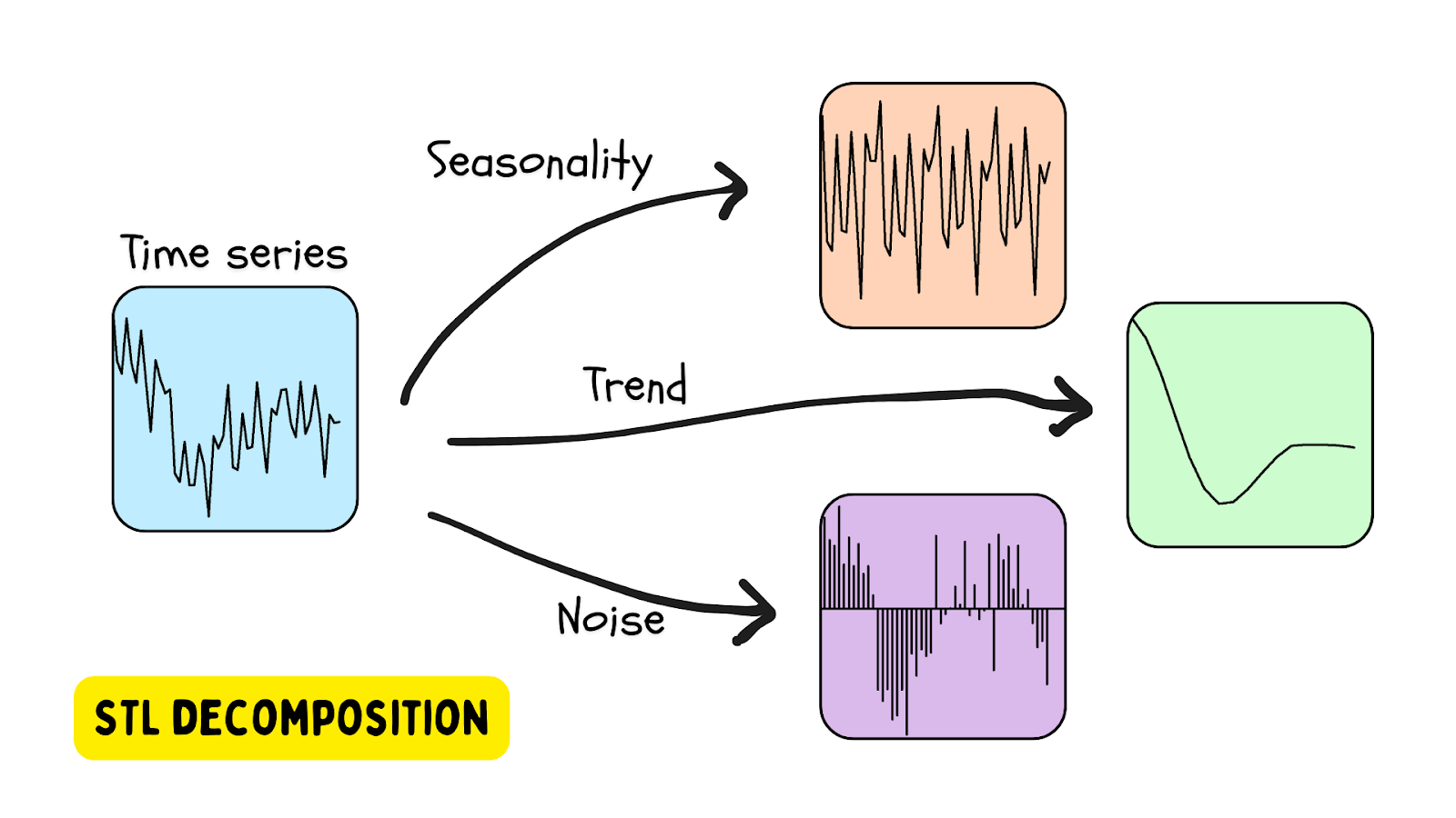
An anomaly is detected when the residual is past a sure threshold.
Utilizing STL decomposition on beehive information
In an earlier weblog put up, we explored anomaly detection in beehives utilizing the OneClassSVM and IsolationForest strategies.
On this tutorial, we’ll analyze beehive information as a time sequence utilizing the STL class supplied by the statsmodels library. To get began, arrange your setting utilizing this file: necessities.txt.
1. Set up the library
Since now we have solely been utilizing the mannequin supplied by Scikit-learn, we might want to set up statsmodels from PyPI. That is straightforward to do in PyCharm.
Go to the Python Bundle window (select the icon on the backside of the left-hand facet of the IDE) and sort in statsmodels within the search field.
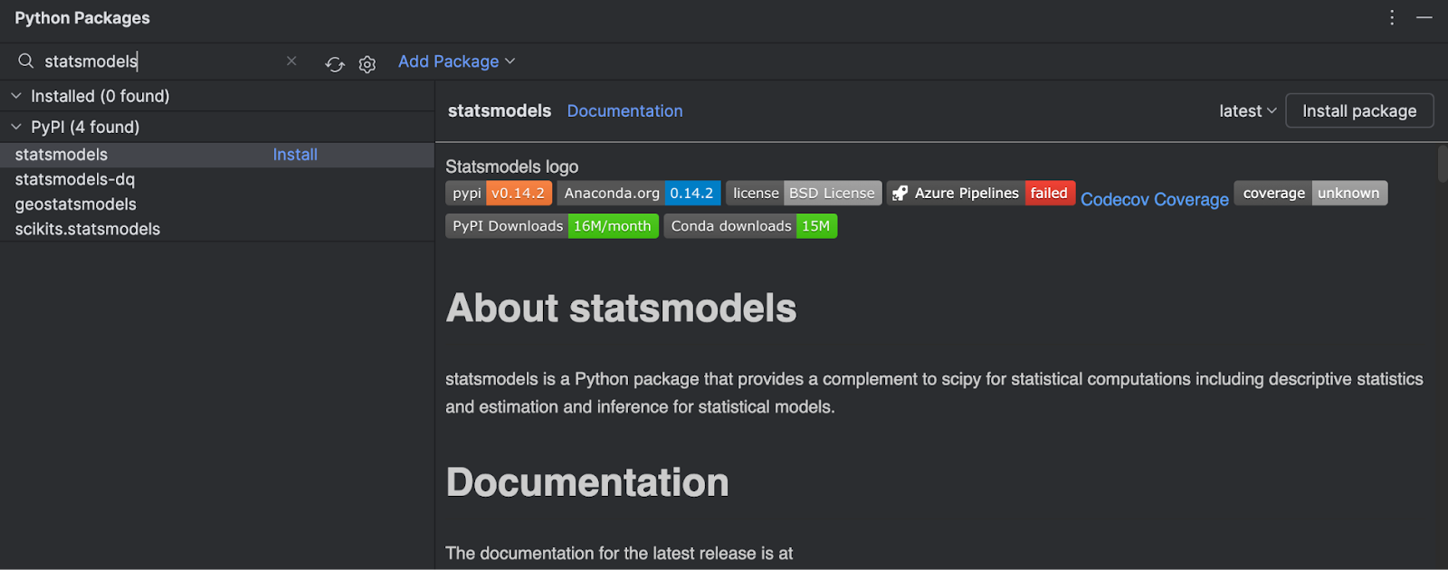
You possibly can see all the details about the package deal on the right-hand facet. To put in it, merely click on Set up package deal.
2. Create a Jupyter pocket book
To analyze the dataset additional, let’s create a Jupyter pocket book to make the most of the instruments that PyCharm’s Jupyter pocket book setting supplies.

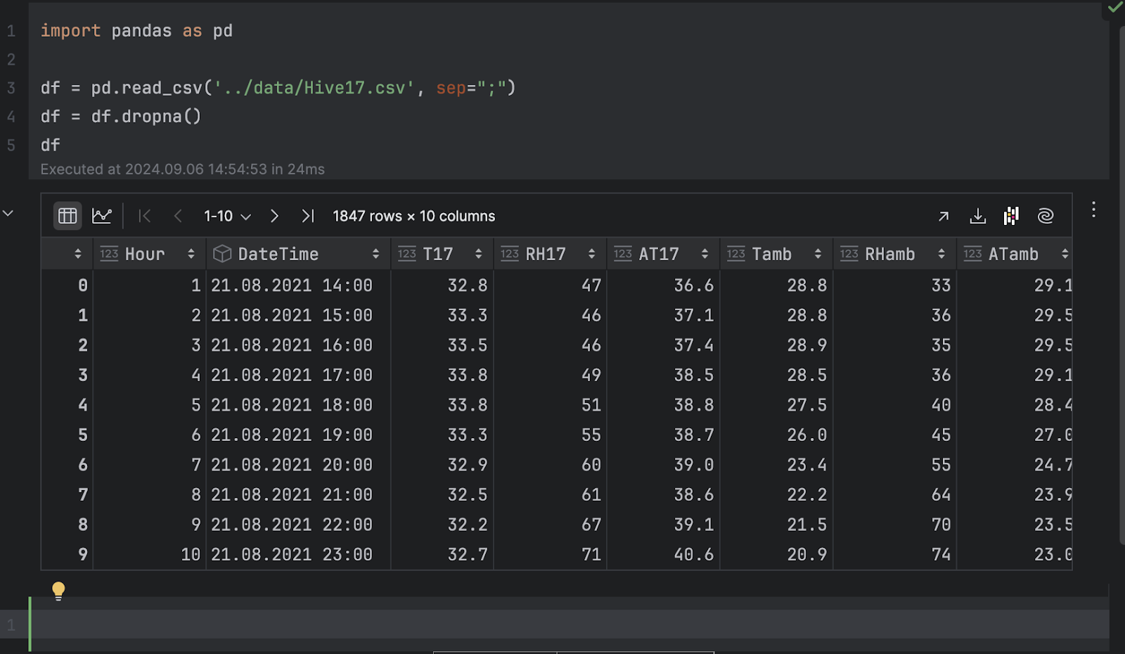
We’ll import pandas and cargo the .csv file.
import pandas as pd

df = pd.read_csv('../information/Hive17.csv', sep=";")
df = df.dropna()
df
3. Examine the information as graphs
Now, we are able to examine the information as graphs. Right here, we want to see the temperature of hive 17 over time. Click on on Chart view within the dataframe inspector after which select T17 because the y-axis within the sequence settings.
When expressed as a time sequence, the temperature has plenty of ups and downs. This means periodic conduct, possible as a result of day-night cycle, so it’s protected to imagine there’s a 24-hour interval for the temperature.
Subsequent, there’s a development of temperature dropping over time. When you examine the DateTime column, you’ll be able to see that the dates vary from August to November. Because the Kaggle web page of the dataset signifies that the information was collected in Turkey, the transition from summer season to fall explains our commentary that the temperature is dropping over time.
4. Time sequence decomposition
To grasp the time sequence and detect anomalies, we’ll carry out STL decomposition, importing the STL class from statsmodels and becoming it with our temperature information.
from statsmodels.tsa.seasonal import STL

stl = STL(df["T17"], interval=24, strong=True)
consequence = stl.match()
We should present a interval for the decomposition to work. As we talked about earlier than, it’s protected to imagine a 24-hour cycle.
Based on the documentation, STL decomposes a time sequence into three parts: development, seasonal, and residual. To get a clearer take a look at the decomposed consequence, we are able to use the built-in plot methodology:
consequence.plot()
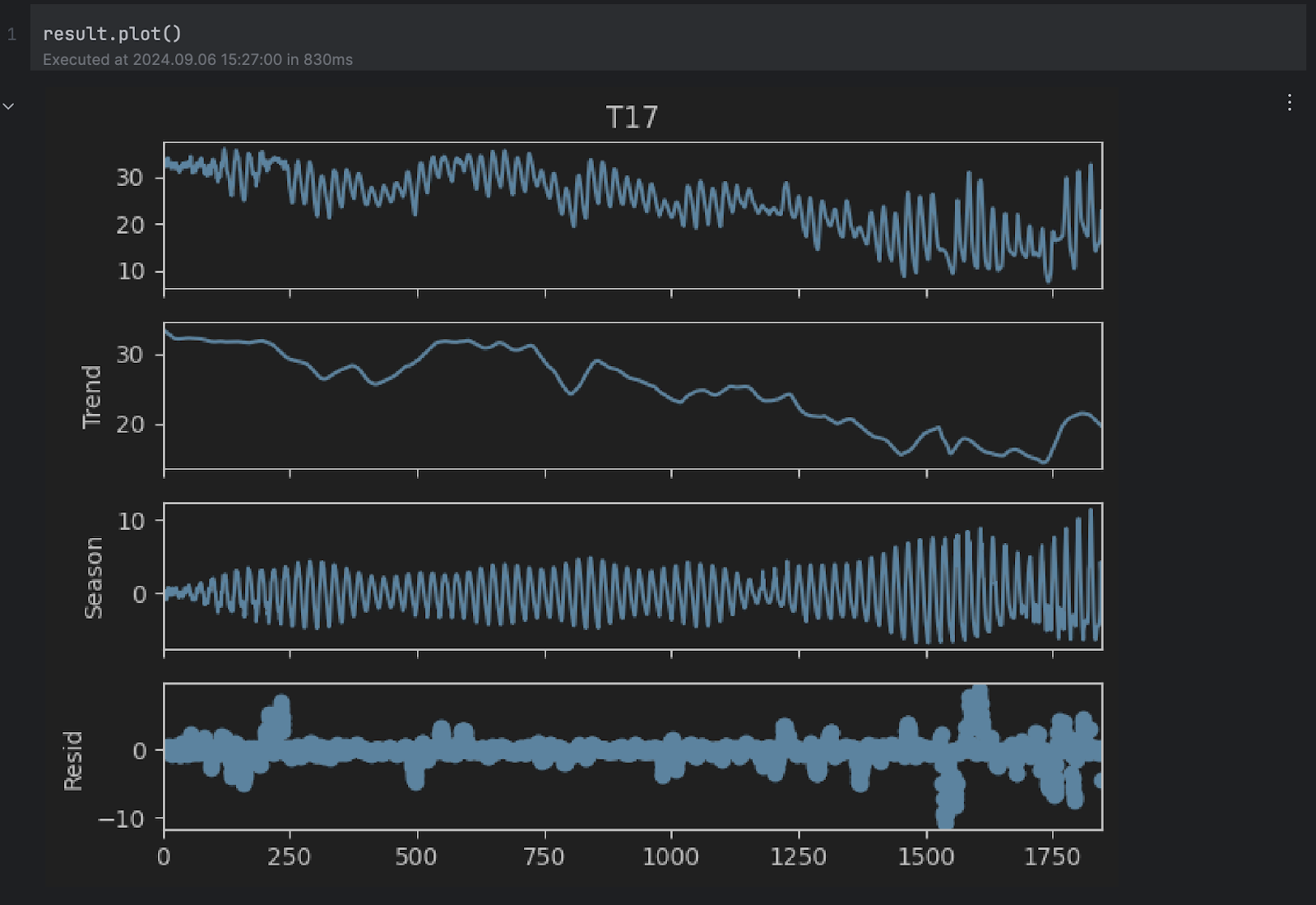
You possibly can see the Development and Season plots appear to align with our assumptions above. Nevertheless, we have an interest within the residual plot on the backside, which is the unique sequence with out the development and seasonal adjustments. Any extraordinarily excessive or low worth within the residual signifies an anomaly.
5. Anomaly threshold
Subsequent, we want to decide what values of the residual we’ll take into account irregular. To try this, we are able to take a look at the residual’s histogram.
consequence.resid.plot.hist()
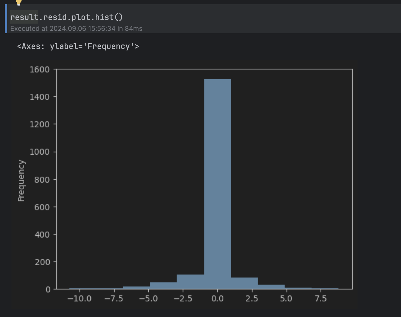
This may be thought of a traditional distribution round 0, with a protracted tail above 5 and under -5, so we’ll set the edge to five.
To point out the anomalies on the unique time sequence, we are able to shade all of them pink within the graph like this:
import matplotlib.pyplot as plt

threshold = 5
anomalies_filter = consequence.resid.apply(lambda x: True if abs(x) > threshold else False)
anomalies = df["T17"][anomalies_filter]

plt.determine(figsize=(14, 8))
plt.scatter(x=anomalies.index, y=anomalies, shade="pink", label="anomalies")
plt.plot(df.index, df['T17'], shade="blue")
plt.title('Temperatures in Hive 17')
plt.xlabel('Hours')
plt.ylabel('Temperature')
plt.legend()
plt.present()
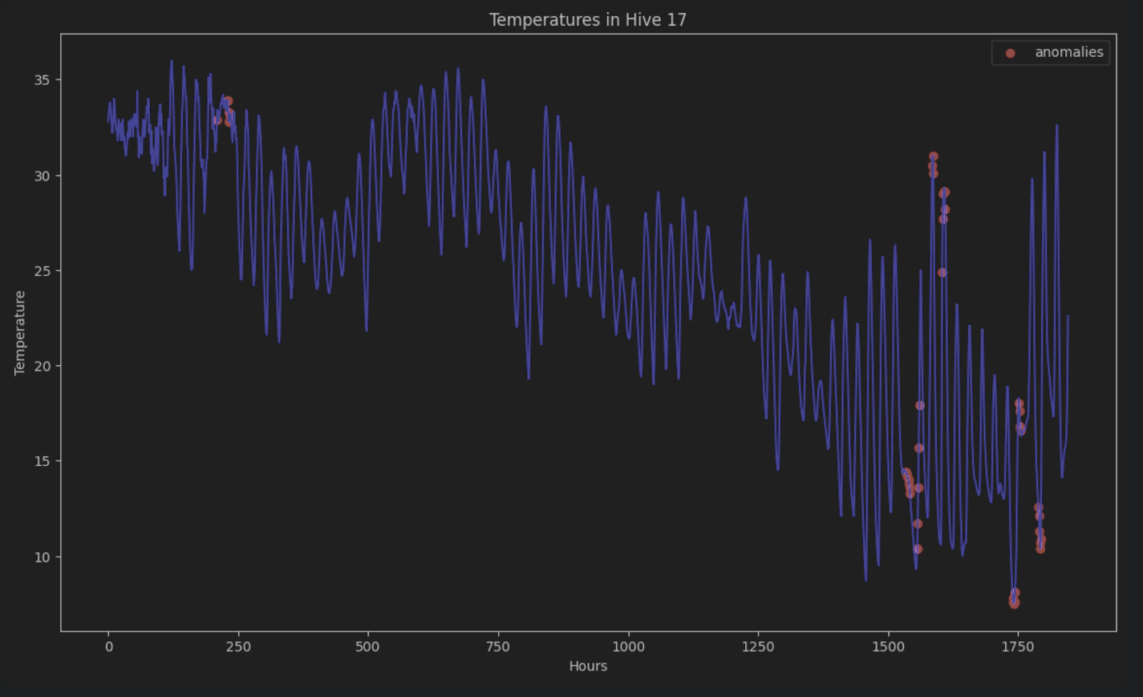
With out STL decomposition, it is vitally arduous to determine these anomalies in a time sequence consisting of durations and tendencies.
LSTM prediction
One other solution to detect anomalies in time sequence information is to do a time sequence prediction on the sequence utilizing deep studying strategies to estimate the end result of knowledge factors. If an estimate may be very totally different from the precise information level, then it could possibly be an indication of anomalous information.
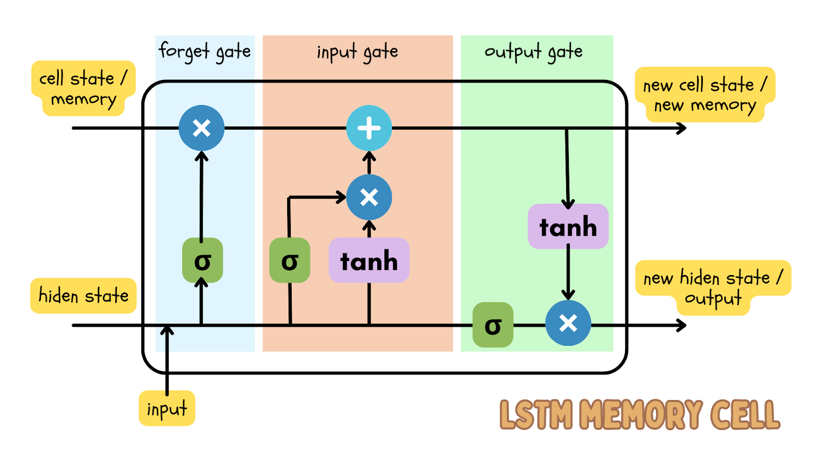
One of many well-liked deep studying algorithms to carry out the prediction of sequential information is the Lengthy short-term reminiscence (LSTM) mannequin, which is a sort of recurrent neural community (RNN). The LSTM mannequin has enter, neglect, and output gates, that are quantity matrices. This ensures essential info is handed on within the subsequent iteration of the information.
Since time sequence information is sequential information, that means the order of knowledge factors is in sequential order and shouldn’t be shuffled, the LSTM mannequin is an efficient deep studying mannequin to foretell the end result at a sure time. This prediction could be in comparison with the precise information and a threshold could be set to find out if the precise information is an anomaly.
Utilizing LSTM prediction on inventory costs
Now let’s begin a brand new Jupyter undertaking to detect any anomalies in Apple’s inventory value over the previous 5 years. The inventory value dataset exhibits probably the most up-to-date information. If you wish to comply with together with the weblog put up, you’ll be able to obtain the dataset we’re utilizing.
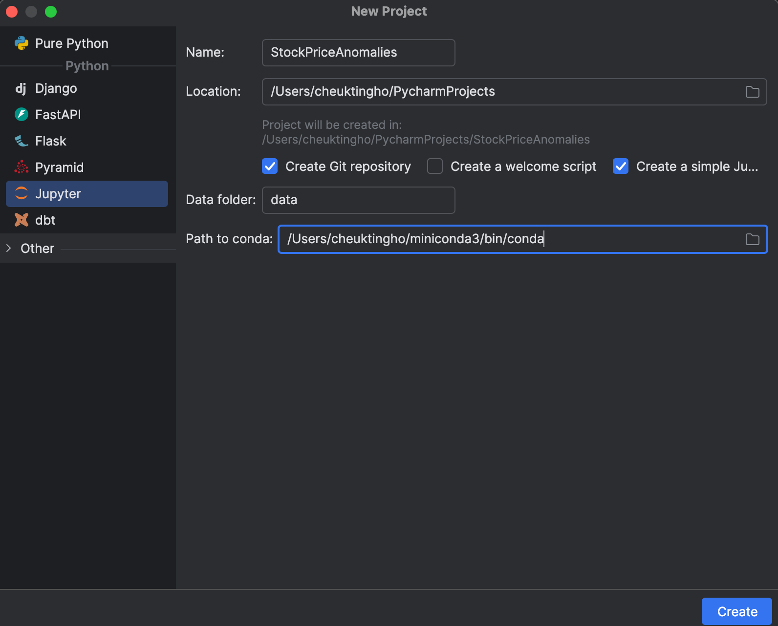
1. Begin a Jupyter undertaking
When beginning a brand new undertaking, you’ll be able to select to create a Jupyter one, which is optimized for information science. Within the New Challenge window, you’ll be able to create a Git repository and decide which conda set up to make use of for managing your setting.
After beginning the undertaking, you will note an instance pocket book. Go forward and begin a brand new Jupyter pocket book for this train.
After that, let’s arrange necessities.txt. We’ll want pandas, matplotlib, and PyTorch, which is called torch on PyPI. Since PyTorch will not be included within the conda setting, PyCharm will inform us that we’re lacking the package deal. To put in the package deal, click on on the lightbulb and choose Set up all lacking packages.
2. Loading and inspecting the information
Subsequent, let’s put our dataset apple_stock_5y.csv within the information folder and cargo it as a pandas DataFrame to examine it.
import pandas as pd

df = pd.read_csv('information/apple_stock_5y.csv')
df
With the interactive desk, we are able to simply see if any information is lacking.
There isn’t any lacking information, however now we have one problem – we want to use the Shut/Final value however it’s not a numeric information sort. Let’s do a conversion and examine our information once more:
df["Close/Last"] = df["Close/Last"].apply(lambda x: float(x[1:]))
df
Now, we are able to examine the value with the interactive desk. Click on on the plot icon on the left and a plot might be created. By default, it makes use of Date because the x-axis and Quantity because the y-axis. Since we want to examine the Shut/Final value, go to the settings by clicking the gear icon on the appropriate and select Shut/Final because the y-axis.
3. Getting ready the coaching information for LSTM
Subsequent, now we have to organize the coaching information for use within the LSTM mannequin. We have to put together a sequence of vectors (function X), every representing a time window, to foretell the subsequent value. The following value will type one other sequence (goal y). Right here we are able to select how massive this time window is with the lookback variable. The next code creates sequences X and y which is able to then be transformed to PyTorch tensors:
import torch

lookback = 5
timeseries = df[["Close/Last"]].values.astype('float32')

X, y = [], []
for i in vary(len(timeseries)-lookback):
    function = timeseries[i:i+lookback]
    goal = timeseries[i+1:i+lookback+1]
    X.append(function)
    y.append(goal)

X = torch.tensor(X)
y = torch.tensor(y)

print(X.form, y.form)
Usually talking, the larger the window, the larger our mannequin might be, for the reason that enter vector is greater. Nevertheless, with an even bigger window, the sequence of inputs might be shorter, so figuring out this lookback window is a balancing act. We’ll begin with 5, however be happy to strive totally different values to see the variations.
4. Construct and practice the mannequin
We will construct the mannequin by creating a category utilizing the nn module in PyTorch earlier than we practice it. The nn module supplies constructing blocks, comparable to totally different neural community layers. On this train, we’ll construct a easy LSTM layer adopted by a linear layer:
import torch.nn as nn

class StockModel(nn.Module):
    def __init__(self):
        tremendous().__init__()
        self.lstm = nn.LSTM(input_size=1, hidden_size=50, num_layers=1, batch_first=True)
        self.linear = nn.Linear(50, 1)
    def ahead(self, x):
        x, _ = self.lstm(x)
        x = self.linear(x)
        return x
Subsequent, we’ll practice our mannequin. Earlier than coaching it, we might want to create an optimizer, a loss operate used to calculate the loss between the expected and precise y values, and a information loader to feed in our coaching information:
import numpy as np
import torch.optim as optim
import torch.utils.information as information

mannequin = StockModel()
optimizer = optim.Adam(mannequin.parameters())
loss_fn = nn.MSELoss()
loader = information.DataLoader(information.TensorDataset(X, y), shuffle=True, batch_size=8)
The info loader can shuffle the enter, as now we have already created the time home windows. This preserves the sequential relationship in every window.
Coaching is finished utilizing a for loop which loops over every epoch. For each 100 epochs, we’ll print out the loss and observe whereas the mannequin converges:
n_epochs = 1000
for epoch in vary(n_epochs):
    mannequin.practice()
    for X_batch, y_batch in loader:
        y_pred = mannequin(X_batch)
        loss = loss_fn(y_pred, y_batch)
        optimizer.zero_grad()
        loss.backward()
        optimizer.step()
    if epoch % 100 != 0:
        proceed
    mannequin.eval()
    with torch.no_grad():
        y_pred = mannequin(X)
        rmse = np.sqrt(loss_fn(y_pred, y))
    print(f"Epoch {epoch}: RMSE {rmse:.4f}")
We begin at 1000 epochs, however the mannequin converges fairly rapidly. Be happy to strive different numbers of epochs for coaching to attain the perfect consequence.
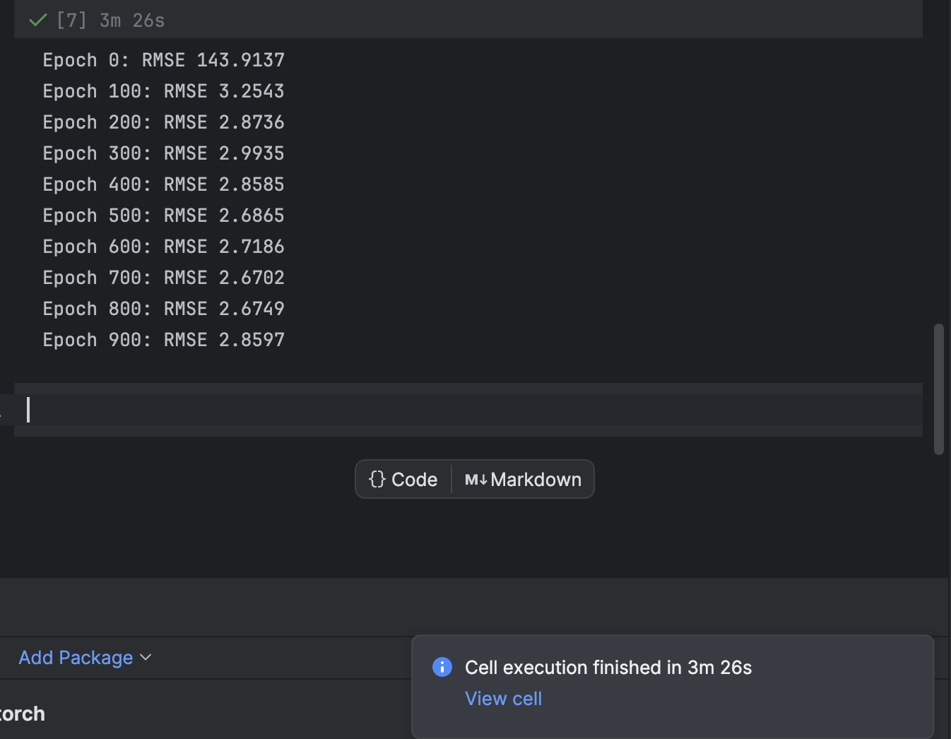
In PyCharm, a cell that requires a while to execute will present a notification about how a lot time stays and a shortcut to the cell. That is very useful when coaching machine studying fashions, particularly deep studying fashions, in Jupyter notebooks.
5. Plot the prediction and discover the errors
Subsequent, we’ll create the prediction and plot it along with the precise time sequence. Be aware that we should create a 2D np sequence to match with the precise time sequence. The precise time sequence might be in blue whereas the expected time sequence might be in pink.
import matplotlib.pyplot as plt

with torch.no_grad():
    pred_series = np.ones_like(timeseries) * np.nan
    pred_series[lookback:] = mannequin(X)[:, -1, :]

plt.plot(timeseries, c="b")
plt.plot(pred_series, c="r")
plt.present()
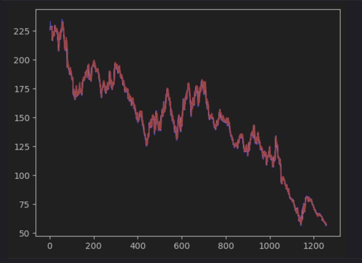
When you observe rigorously, you will note that the prediction and the precise values don’t align completely. Nevertheless, many of the predictions do a great job.
To examine the errors carefully, we are able to create an error sequence and use the interactive desk to look at them. We’re utilizing absolutely the error this time.
error = abs(timeseries-pred_series)
error
Use the settings to create a histogram with the worth of absolutely the error because the x-axis and the rely of the worth because the y-axis.
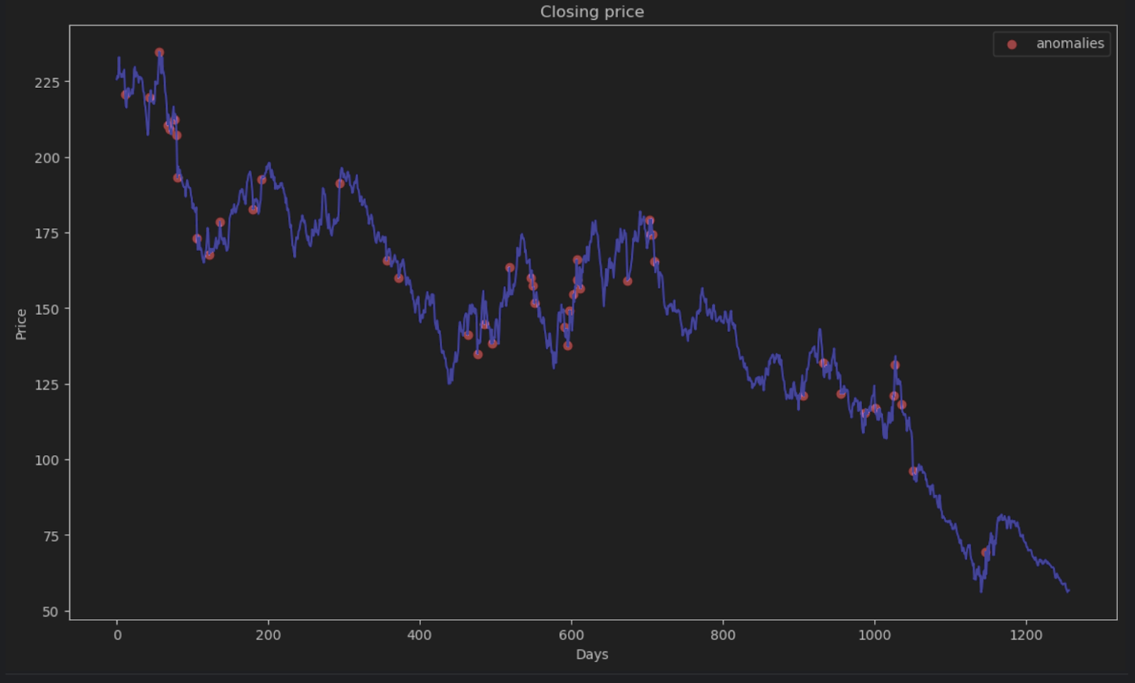
6. Resolve on the anomaly threshold and visualize
Many of the factors can have an absolute error of lower than 6, so we are able to set that because the anomaly threshold. Just like what we did for the beehive anomalies, we are able to plot the anomalous information factors within the graph.
threshold = 6
error_series = pd.Collection(error.flatten())
price_series = pd.Collection(timeseries.flatten())

anomalies_filter = error_series.apply(lambda x: True if x > threshold else False)
anomalies = price_series[anomalies_filter]

plt.determine(figsize=(14, 8))
plt.scatter(x=anomalies.index, y=anomalies, shade="pink", label="anomalies")
plt.plot(df.index, timeseries, shade="blue")
plt.title('Closing value')
plt.xlabel('Days')
plt.ylabel('Value')
plt.legend()
plt.present()
Abstract
Time sequence information is a typical type of information utilized in many functions together with enterprise and scientific analysis. Because of the sequential nature of time sequence information, particular strategies and algorithms are used to assist decide anomalies in it. On this weblog put up, we demonstrated learn how to determine anomalies utilizing STL decomposition to get rid of seasonalities and tendencies. We now have additionally demonstrated learn how to use deep studying and the LSTM mannequin to check the expected estimate and the precise information with a purpose to decide anomalies.
Detect anomalies utilizing PyCharm
With the Jupyter undertaking in PyCharm Skilled, you’ll be able to manage your anomaly detection undertaking with plenty of information recordsdata and notebooks simply. Graphs output could be generated to examine anomalies and plots are very accessible in PyCharm. Different options, comparable to auto-complete solutions, make navigating all of the Scikit-learn fashions and Matplotlib plot settings a blast.
Energy up your information science tasks through the use of PyCharm, and try the information science options supplied to streamline your information science workflow.

Subscribe to PyCharm Weblog updates
