


After considering it over, I feel I would love to do two (or perhaps three) follow-up posts. The primary follow-up put up, at the moment, will concentrate on some methods to visualise the place a curve in Lab house goes out-of-gamut for sRGB. Subsequent, I will discover methods to switch the approach I demonstrated beforehand with the intention to keep away from out-of-gamut colours.
Right here is the colormap I confirmed within the 09-Could-2006 put up:
theta = linspace(0, pi/2, 256).’;
L = linspace(0, 100, 256).’;
Show the colormap:
fig.Place(4) = fig.Place(4)/3;

This led me to discover alternative ways to visualise which colours in a Lab curve are out of gamut. (Notice that this dialogue assumes that we’re speaking about sRGB, which is the default coloration house utilized by lab2rgb.) The very first thing I attempted was so as to add marks to the displayed colormap to point which colours are out-of-gamut. This subsequent block of code finds all of the contiguous segments of out-of-gamut colours within the colormap.
out_of_gamut_mask = any(rgb > 1,2) | any(rgb < 0,2);
d = diff([0 ; out_of_gamut_mask ; 0]);
The values of first and final above imply that the Lab colours lab(1:61,:) and lab(211:256,:) are out of the sRGB gamut. Now use these numbers so as to add gamut alarm indicators (crimson bars) to the displayed colormap.
plot(ax,x,y,“r”,LineWidth = 5)
maintain off

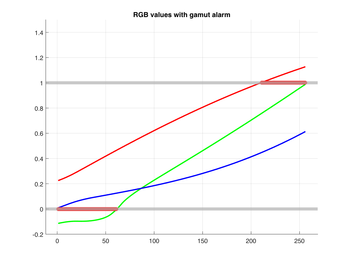
One other visualization method is to plot the crimson, inexperienced, and blue coloration part values returned by lab2rgb and present the place these values are too excessive or too low.
xlim([1 – 0.05*height(rgb), 1.05*height(rgb)]);
y1 = min(-0.2,ax.YLim(1));
y2 = max(1.2,ax.YLim(2));
yline(0, LineWidth = 5, Shade = [0.7 0.7 0.7])
yline(1, LineWidth = 5, Shade = [0.7 0.7 0.7])
too_high = any(rgb > 1,2);
plot(okay,ones(dimension(okay)),‘r*’,MarkerSize = 6)
too_low = any(rgb < 0,2);
plot(okay,zeros(dimension(okay)),‘r*’,MarkerSize = 6)
title(“RGB values with gamut alarm”)
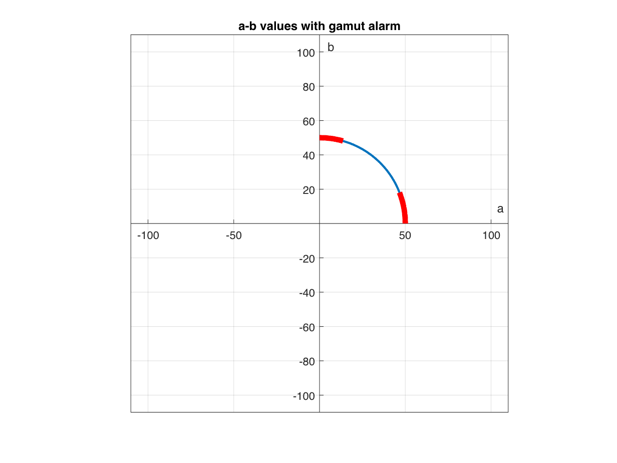
Subsequent I need to present the a and b values for the out-of-gamut Lab curve colours.
ax.XAxisLocation = “origin”;
ax.YAxisLocation = “origin”;
plot(x,y,“r”,LineWidth = 5)
title(“a-b values with gamut alarm”)
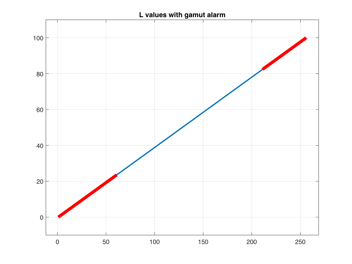
Lastly, I need to present the L values for the out-of-gamut Lab curve colours.
xlim([1 – 0.05*height(lab), 1.05*height(lab)]);
plot(x,y,“r”,LineWidth = 5)
title(“L values with gamut alarm”)
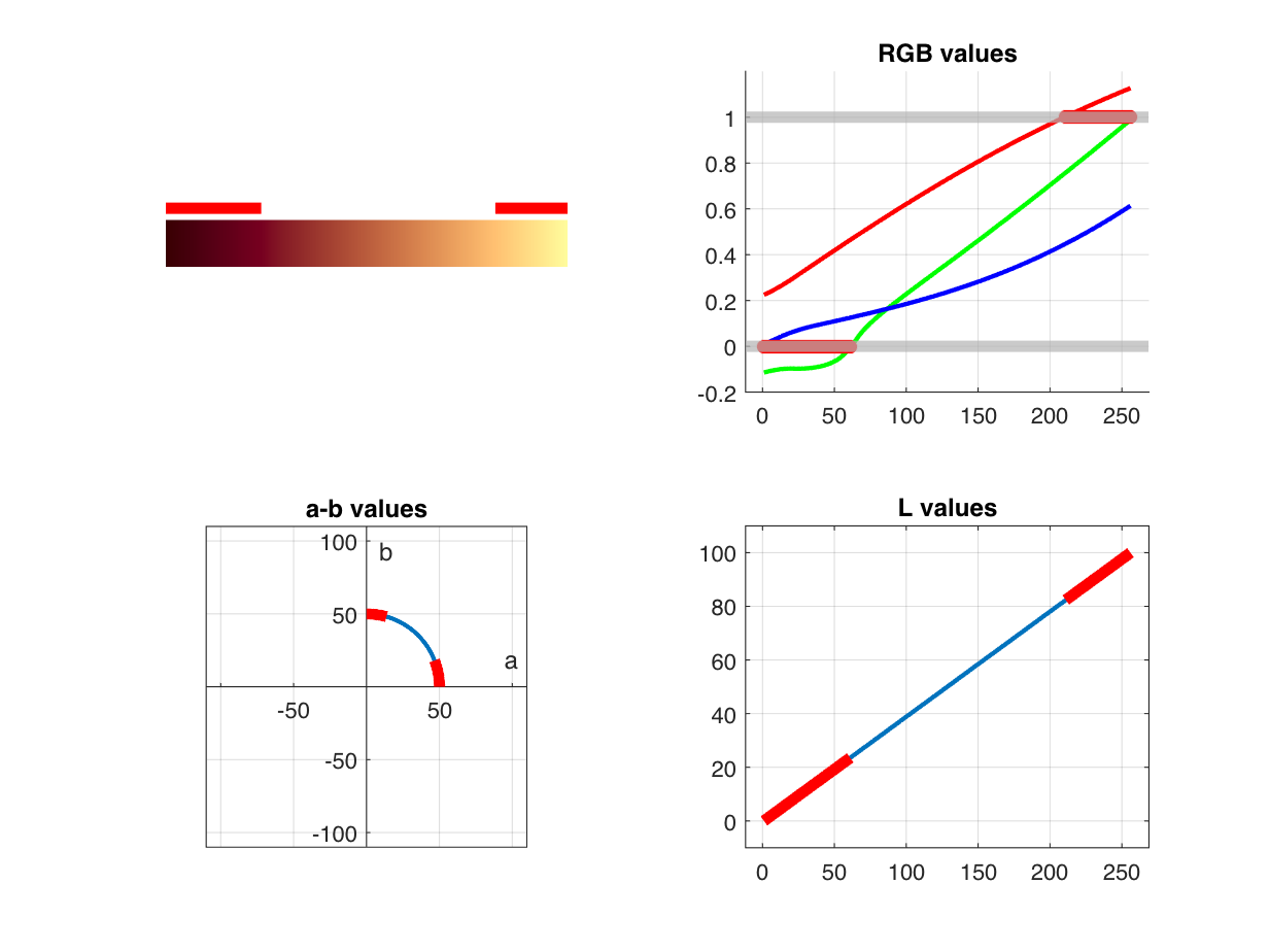
I created some utility capabilities that generate these completely different plots. They’re on the finish of this put up. I will end up through the use of tiledlayout to mix all 4 plots in a single determine.
plotLabColormapWithGamutAlarm(lab)
plotLabRGBColorsWithGamutAlarm(lab)
plotABWithGamutAlarm(lab)
title(“L values”)
Utility Capabilities
operate plotLabColormapWithGamutAlarm(lab)
[first,last] = outOfGamutSegments(lab);
plot(ax,x,y,‘r’,LineWidth = 5)
operate plotLabRGBColorsWithGamutAlarm(lab)
xlim(ax,[1 – 0.05*height(rgb), 1.05*height(rgb)]);
y1 = min(-0.2,ax.YLim(1));
y2 = max(1.2,ax.YLim(2));
yline(ax,0, LineWidth = 5, Shade = [0.7 0.7 0.7])
yline(ax,1, LineWidth = 5, Shade = [0.7 0.7 0.7])
too_high = any(rgb > 1,2);
plot(ax,okay,ones(dimension(okay)),‘r*’,MarkerSize = 6)
too_low = any(rgb < 0,2);
plot(ax,okay,zeros(dimension(okay)),‘r*’,MarkerSize = 6)
operate plotABWithGamutAlarm(lab)
plot(ax,lab(:,2),lab(:,3));
ax.XAxisLocation = “origin”;
ax.YAxisLocation = “origin”;
[first,last] = outOfGamutSegments(lab);
plot(ax,x,y,‘r’,LineWidth = 5)
operate plotLWithGamutAlarm(lab)
xlim(ax,[1 – 0.05*height(lab), 1.05*height(lab)]);
[first,last] = outOfGamutSegments(lab);
plot(ax,x,y,‘r’,LineWidth = 5)
operate [first,last] = outOfGamutSegments(lab)
out_of_gamut_mask = any(rgb > 1,2) | any(rgb < 0,2);
d = diff([0 ; out_of_gamut_mask ; 0]);
final = discover(d == -1) – 1;