



These are all of the packages you’ll want for Python statistics calculations. Often, you received’t use Python’s built-in math package deal, nevertheless it’ll be helpful on this tutorial. Later, you’ll import matplotlib.pyplot for information visualization.
Let’s create some information to work with. You’ll begin with Python lists that include some arbitrary numeric information:
Now you may have the lists x and x_with_nan. They’re nearly the identical, with the distinction that x_with_nan incorporates a nan worth. It’s vital to grasp the conduct of the Python statistics routines after they come throughout a not-a-number worth (nan). In information science, lacking values are widespread, and also you’ll usually change them with nan.
Now, create np.ndarray and pd.Sequence objects that correspond to x and x_with_nan:
You now have two NumPy arrays (y and y_with_nan) and two pandas Sequence (z and z_with_nan). All of those are 1D sequences of values.
You’ll be able to optionally specify a label for every worth in z and z_with_nan.
Measures of Central Tendency
The measures of central tendency present the central or center values of datasets. There are a number of definitions of what’s thought of to be the middle of a dataset. On this tutorial, you’ll learn to establish and calculate these measures of central tendency:
- Imply
- Weighted imply
- Geometric imply
- Harmonic imply
- Median
- Mode
Imply
The pattern imply, additionally known as the pattern arithmetic imply or just the common, is the arithmetic common of all of the objects in a dataset. The imply of a dataset 𝑥 is mathematically expressed as Σᵢ𝑥ᵢ/𝑛, the place 𝑖 = 1, 2, …, 𝑛. In different phrases, it’s the sum of all the weather 𝑥ᵢ divided by the variety of objects within the dataset 𝑥.
This determine illustrates the imply of a pattern with 5 information factors:
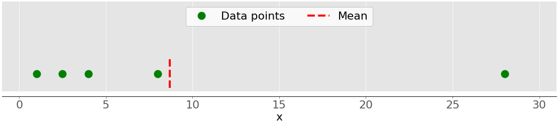
The inexperienced dots signify the information factors 1, 2.5, 4, 8, and 28. The purple dashed line is their imply, or (1 + 2.5 + 4 + 8 + 28) / 5 = 8.7.
You’ll be able to calculate the imply with pure Python utilizing sum() and len(), with out importing libraries:
Though that is clear and stylish, you can too apply built-in Python statistics features:
You’ve known as the features imply() and fmean() from the built-in Python statistics library and received the identical end result as you probably did with pure Python. fmean() is launched in Python 3.8 as a sooner different to imply(). It at all times returns a floating-point quantity.
Nevertheless, if there are nan values amongst your information, then statistics.imply() and statistics.fmean() will return nan because the output:
This result’s per the conduct of sum(), as a result of sum(x_with_nan) additionally returns nan.
When you use NumPy, then you will get the imply with np.imply():
Within the instance above, imply() is a perform, however you should utilize the corresponding technique .imply() as nicely:
The perform imply() and technique .imply() from NumPy return the identical end result as statistics.imply(). That is additionally the case when there are nan values amongst your information:
You usually don’t must get a nan worth because of this. When you favor to disregard nan values, then you should utilize np.nanmean():
nanmean() merely ignores all nan values. It returns the identical worth as imply() for those who had been to use it to the dataset with out the nan values.
pd.Sequence objects even have the strategy .imply():
As you’ll be able to see, it’s used equally as within the case of NumPy. Nevertheless, .imply() from pandas ignores nan values by default:
This conduct is the results of the default worth of the non-obligatory parameter skipna. You’ll be able to change this parameter to change the conduct.
Weighted Imply
The weighted imply, additionally known as the weighted arithmetic imply or weighted common, is a generalization of the arithmetic imply that lets you outline the relative contribution of every information level to the end result.
You outline one weight 𝑤ᵢ for every information level 𝑥ᵢ of the dataset 𝑥, the place 𝑖 = 1, 2, …, 𝑛 and 𝑛 is the variety of objects in 𝑥. Then, you multiply every information level with the corresponding weight, sum all of the merchandise, and divide the obtained sum with the sum of weights: Σᵢ(𝑤ᵢ𝑥ᵢ) / Σᵢ𝑤ᵢ.
Observe: It’s handy (and often the case) that every one weights are nonnegative, 𝑤ᵢ ≥ 0, and that their sum is the same as one, or Σᵢ𝑤ᵢ = 1.
The weighted imply could be very useful if you want the imply of a dataset containing objects that happen with given relative frequencies. For instance, say that you’ve got a set wherein 20% of all objects are equal to 2, 50% of the objects are equal to 4, and the remaining 30% of the objects are equal to eight. You’ll be able to calculate the imply of such a set like this:
Right here, you’re taking the frequencies into consideration with the weights. With this technique, you don’t must know the overall variety of objects.
You’ll be able to implement the weighted imply in pure Python by combining sum() with both vary() or zip():
Once more, it is a clear and stylish implementation the place you don’t must import any libraries.
Nevertheless, if in case you have massive datasets, then NumPy is probably going to offer a greater answer. You should utilize np.common() to get the weighted imply of NumPy arrays or pandas Sequence:
The end result is identical as within the case of the pure Python implementation. You can even use this technique on atypical lists and tuples.
One other answer is to make use of the element-wise product w * y with np.sum() or .sum():
That’s it! You’ve calculated the weighted imply.
Nevertheless, watch out in case your dataset incorporates nan values:
On this case, common() returns nan, which is per np.imply().
Harmonic Imply
The harmonic imply is the reciprocal of the imply of the reciprocals of all objects within the dataset: 𝑛 / Σᵢ(1/𝑥ᵢ), the place 𝑖 = 1, 2, …, 𝑛 and 𝑛 is the variety of objects within the dataset 𝑥. One variant of the pure Python implementation of the harmonic imply is that this:
It’s fairly completely different from the worth of the arithmetic imply for a similar information x, which you calculated to be 8.7.
You can even calculate this measure with statistics.harmonic_mean():
The instance above exhibits one implementation of statistics.harmonic_mean(). When you’ve got a nan worth in a dataset, then it’ll return nan. If there’s not less than one 0, then it’ll return 0. When you present not less than one unfavorable quantity, then you definitely’ll get statistics.StatisticsError:
Maintain these three eventualities in thoughts if you’re utilizing this technique!
A 3rd technique to calculate the harmonic imply is to make use of scipy.stats.hmean():
Once more, it is a fairly simple implementation. Nevertheless, in case your dataset incorporates nan, 0, a unfavorable quantity, or something however constructive numbers, then you definitely’ll get a ValueError!
Geometric Imply
The geometric imply is the 𝑛-th root of the product of all 𝑛 parts 𝑥ᵢ in a dataset 𝑥: ⁿ√(Πᵢ𝑥ᵢ), the place 𝑖 = 1, 2, …, 𝑛. The next determine illustrates the arithmetic, harmonic, and geometric technique of a dataset:
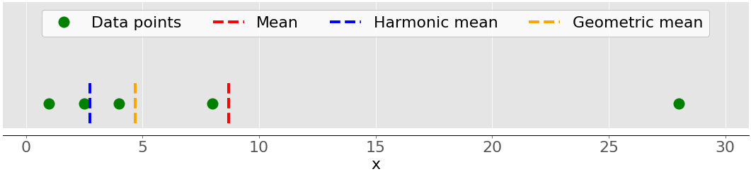
Once more, the inexperienced dots signify the information factors 1, 2.5, 4, 8, and 28. The purple dashed line is the imply. The blue dashed line is the harmonic imply, and the yellow dashed line is the geometric imply.
You’ll be able to implement the geometric imply in pure Python like this:
As you’ll be able to see, the worth of the geometric imply, on this case, differs considerably from the values of the arithmetic (8.7) and harmonic (2.76) means for a similar dataset x.
Python 3.8 launched statistics.geometric_mean(), which converts all values to floating-point numbers and returns their geometric imply:
You’ve received the identical end result as within the earlier instance, however with a minimal rounding error.
When you cross information with nan values, then statistics.geometric_mean() will behave like most comparable features and return nan:
Certainly, that is per the conduct of statistics.imply(), statistics.fmean(), and statistics.harmonic_mean(). If there’s a zero or unfavorable quantity amongst your information, then statistics.geometric_mean() will elevate the statistics.StatisticsError.
You can even get the geometric imply with scipy.stats.gmean():
You obtained the identical end result as with the pure Python implementation.
When you’ve got nan values in a dataset, then gmean() will return nan. If there’s not less than one 0, then it’ll return 0.0 and provides a warning. When you present not less than one unfavorable quantity, then you definitely’ll get nan and the warning.
Median
The pattern median is the center aspect of a sorted dataset. The dataset could be sorted in rising or reducing order. If the variety of parts 𝑛 of the dataset is odd, then the median is the worth on the center place: 0.5(𝑛 + 1). If 𝑛 is even, then the median is the arithmetic imply of the 2 values within the center, that’s, the objects on the positions 0.5𝑛 and 0.5𝑛 + 1.
For instance, if in case you have the information factors 2, 4, 1, 8, and 9, then the median worth is 4, which is in the course of the sorted dataset (1, 2, 4, 8, 9). If the information factors are 2, 4, 1, and eight, then the median is 3, which is the common of the 2 center parts of the sorted sequence (2 and 4). The next determine illustrates this:
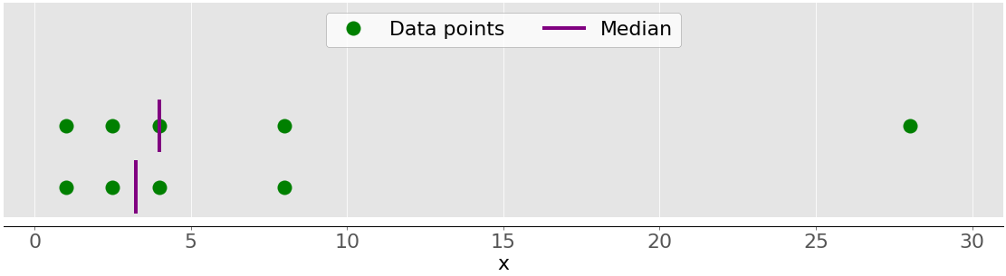
The info factors are the inexperienced dots, and the purple strains present the median for every dataset. The median worth for the higher dataset (1, 2.5, 4, 8, and 28) is 4. When you take away the outlier 28 from the decrease dataset, then the median turns into the arithmetic common between 2.5 and 4, which is 3.25.
The determine beneath exhibits each the imply and median of the information factors 1, 2.5, 4, 8, and 28:
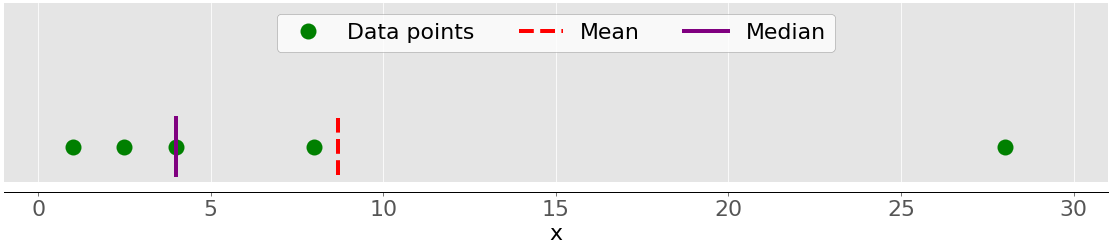
Once more, the imply is the purple dashed line, whereas the median is the purple line.
The primary distinction between the conduct of the imply and median is said to dataset outliers or extremes. The imply is closely affected by outliers, however the median solely depends upon outliers both barely or by no means. Think about the next determine:
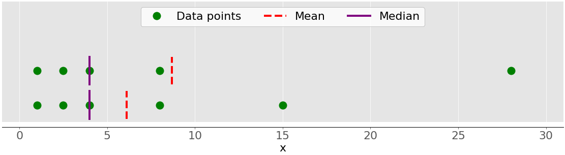
The higher dataset once more has the objects 1, 2.5, 4, 8, and 28. Its imply is 8.7, and the median is 4, as you noticed earlier. The decrease dataset exhibits what’s happening if you transfer the rightmost level with the worth 28:
- When you enhance its worth (transfer it to the fitting), then the imply will rise, however the median worth received’t ever change.
- When you lower its worth (transfer it to the left), then the imply will drop, however the median will stay the identical till the worth of the transferring level is bigger than or equal to 4.
You’ll be able to examine the imply and median as one technique to detect outliers and asymmetry in your information. Whether or not the imply worth or the median worth is extra helpful to you depends upon the context of your explicit drawback.
Right here is one among many doable pure Python implementations of the median:
Two most vital steps of this implementation are as follows:
- Sorting the weather of the dataset
- Discovering the center aspect(s) within the sorted dataset
You may get the median with statistics.median():
The sorted model of x is [1, 2.5, 4, 8.0, 28.0], so the aspect within the center is 4. The sorted model of x[:-1], which is x with out the final merchandise 28.0, is [1, 2.5, 4, 8.0]. Now, there are two center parts, 2.5 and 4. Their common is 3.25.
median_low() and median_high() are two extra features associated to the median within the Python statistics library. They at all times return a component from the dataset:
- If the variety of parts is odd, then there’s a single center worth, so these features behave identical to
median(). - If the variety of parts is even, then there are two center values. On this case,
median_low()returns the decrease andmedian_high()the upper center worth.
You should utilize these features simply as you’d use median():
Once more, the sorted model of x[:-1] is [1, 2.5, 4, 8.0]. The 2 parts within the center are 2.5 (low) and 4 (excessive).
In contrast to most different features from the Python statistics library, median(), median_low(), and median_high() don’t return nan when there are nan values among the many information factors:
Watch out for this conduct as a result of it may not be what you need!
You can even get the median with np.median():
You’ve obtained the identical values with statistics.median() and np.median().
Nevertheless, if there’s a nan worth in your dataset, then np.median() points the RuntimeWarning and returns nan. If this conduct just isn’t what you need, then you should utilize nanmedian() to disregard all nan values:
The obtained outcomes are the identical as with statistics.median() and np.median() utilized to the datasets x and y.
pandas Sequence objects have the strategy .median() that ignores nan values by default:
The conduct of .median() is per .imply() in pandas. You’ll be able to change this conduct with the non-obligatory parameter skipna.
Mode
The pattern mode is the worth within the dataset that happens most ceaselessly. If there isn’t a single such worth, then the set is multimodal because it has a number of modal values. For instance, within the set that incorporates the factors 2, 3, 2, 8, and 12, the quantity 2 is the mode as a result of it happens twice, not like the opposite objects that happen solely as soon as.
That is how one can get the mode with pure Python:
You utilize u.rely() to get the variety of occurrences of every merchandise in u. The merchandise with the maximal variety of occurrences is the mode. Observe that you simply don’t have to make use of set(u). As a substitute, you may change it with simply u and iterate over the complete listing.
Observe: set(u) returns a Python set with all distinctive objects in u. You should utilize this trick to optimize working with bigger information, particularly if you anticipate to see a variety of duplicates.
You’ll be able to get hold of the mode with statistics.mode() and statistics.multimode():
As you’ll be able to see, mode() returned a single worth, whereas multimode() returned the listing that incorporates the end result. This isn’t the one distinction between the 2 features, although. If there’s multiple modal worth, then mode() raises StatisticsError, whereas multimode() returns the listing with all modes:
It is best to pay particular consideration to this situation and watch out if you’re selecting between these two features.
statistics.mode() and statistics.multimode() deal with nan values as common values and may return nan because the modal worth:
Within the first instance above, the quantity 2 happens twice and is the modal worth. Within the second instance, nan is the modal worth because it happens twice, whereas the opposite values happen solely as soon as.
Observe: statistics.multimode() is launched in Python 3.8.
You can even get the mode with scipy.stats.mode():
This perform returns the article with the modal worth and the variety of occasions it happens. If there are a number of modal values within the dataset, then solely the smallest worth is returned.
You may get the mode and its variety of occurrences with dot notation:
This code makes use of .mode to return the smallest mode (12) within the array v and .rely to return the variety of occasions it happens (3). scipy.stats.mode() can be versatile with nan values. It lets you outline desired conduct with the non-obligatory parameter nan_policy. This parameter can tackle the values "propagate", "elevate" (an error), or "omit".
pandas Sequence objects have the strategy .mode() that handles multimodal values nicely and ignores nan values by default:
As you’ll be able to see, .mode() returns a brand new pd.Sequence that holds all modal values. If you would like .mode() to take nan values into consideration, then simply cross the non-obligatory argument dropna=False.
Measures of Variability
The measures of central tendency aren’t enough to explain information. You’ll additionally want the measures of variability that quantify the unfold of knowledge factors. On this part, you’ll learn to establish and calculate the next variability measures:
- Variance
- Normal deviation
- Skewness
- Percentiles
- Ranges
Variance
The pattern variance quantifies the unfold of the information. It exhibits numerically how far the information factors are from the imply. You’ll be able to categorical the pattern variance of the dataset 𝑥 with 𝑛 parts mathematically as 𝑠² = Σᵢ(𝑥ᵢ − imply(𝑥))² / (𝑛 − 1), the place 𝑖 = 1, 2, …, 𝑛 and imply(𝑥) is the pattern imply of 𝑥. If you wish to perceive deeper why you divide the sum with 𝑛 − 1 as an alternative of 𝑛, then you’ll be able to dive deeper into Bessel’s correction.
The next determine exhibits you why it’s vital to contemplate the variance when describing datasets:
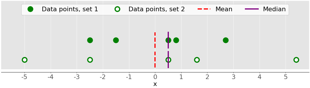
There are two datasets on this determine:
- Inexperienced dots: This dataset has a smaller variance or a smaller common distinction from the imply. It additionally has a smaller vary or a smaller distinction between the biggest and smallest merchandise.
- White dots: This dataset has a bigger variance or a bigger common distinction from the imply. It additionally has an even bigger vary or an even bigger distinction between the biggest and smallest merchandise.
Observe that these two datasets have the identical imply and median, despite the fact that they seem to vary considerably. Neither the imply nor the median can describe this distinction. That’s why you want the measures of variability.
Right here’s how one can calculate the pattern variance with pure Python:
This method is enough and calculates the pattern variance nicely. Nevertheless, the shorter and extra elegant answer is to name the present perform statistics.variance():
You’ve obtained the identical end result for the variance as above. variance() can keep away from calculating the imply for those who present the imply explicitly because the second argument: statistics.variance(x, mean_).
When you’ve got nan values amongst your information, then statistics.variance() will return nan:
This conduct is per imply() and most different features from the Python statistics library.
You can even calculate the pattern variance with NumPy. It is best to use the perform np.var() or the corresponding technique .var():
It’s crucial to specify the parameter ddof=1. That’s the way you set the delta levels of freedom to 1. This parameter permits the right calculation of 𝑠², with (𝑛 − 1) within the denominator as an alternative of 𝑛.
When you’ve got nan values within the dataset, then np.var() and .var() will return nan:
That is per np.imply() and np.common(). If you wish to skip nan values, then it is best to use np.nanvar():
np.nanvar() ignores nan values. It additionally wants you to specify ddof=1.
pd.Sequence objects have the strategy .var() that skips nan values by default:
It additionally has the parameter ddof, however its default worth is 1, so you’ll be able to omit it. If you would like a unique conduct associated to nan values, then use the non-obligatory parameter skipna.
You calculate the inhabitants variance equally to the pattern variance. Nevertheless, it’s important to use 𝑛 within the denominator as an alternative of 𝑛 − 1: Σᵢ(𝑥ᵢ − imply(𝑥))² / 𝑛. On this case, 𝑛 is the variety of objects in the complete inhabitants. You may get the inhabitants variance much like the pattern variance, with the next variations:
- Substitute
(n - 1)withnwithin the pure Python implementation. - Use
statistics.pvariance()as an alternative ofstatistics.variance(). - Specify the parameter
ddof=0for those who use NumPy or pandas. In NumPy, you’ll be able to omitddofas a result of its default worth is0.
Observe that it is best to at all times concentrate on whether or not you’re working with a pattern or the complete inhabitants everytime you’re calculating the variance!
Normal Deviation
The pattern commonplace deviation is one other measure of knowledge unfold. It’s linked to the pattern variance, as commonplace deviation, 𝑠, is the constructive sq. root of the pattern variance. The usual deviation is usually extra handy than the variance as a result of it has the identical unit as the information factors. When you get the variance, you’ll be able to calculate the usual deviation with pure Python:
Though this answer works, you can too use statistics.stdev():
In fact, the end result is identical as earlier than. Like variance(), stdev() doesn’t calculate the imply for those who present it explicitly because the second argument: statistics.stdev(x, mean_).
You may get the usual deviation with NumPy in nearly the identical means. You should utilize the perform std() and the corresponding technique .std() to calculate the usual deviation. If there are nan values within the dataset, then they’ll return nan. To disregard nan values, it is best to use np.nanstd(). You utilize std(), .std(), and nanstd() from NumPy as you’d use var(), .var(), and nanvar():
Don’t overlook to set the delta levels of freedom to 1!
pd.Sequence objects even have the strategy .std() that skips nan by default:
The parameter ddof defaults to 1, so you’ll be able to omit it. Once more, if you wish to deal with nan values otherwise, then apply the parameter skipna.
The inhabitants commonplace deviation refers back to the total inhabitants. It’s the constructive sq. root of the inhabitants variance. You’ll be able to calculate it identical to the pattern commonplace deviation, with the next variations:
- Discover the sq. root of the inhabitants variance within the pure Python implementation.
- Use
statistics.pstdev()as an alternative ofstatistics.stdev(). - Specify the parameter
ddof=0for those who use NumPy or pandas. In NumPy, you’ll be able to omitddofas a result of its default worth is0.
As you’ll be able to see, you’ll be able to decide the usual deviation in Python, NumPy, and pandas in nearly the identical means as you identify the variance. You utilize completely different however analogous features and strategies with the identical arguments.
Skewness
The pattern skewness measures the asymmetry of a knowledge pattern.
There are a number of mathematical definitions of skewness. One widespread expression to calculate the skewness of the dataset 𝑥 with 𝑛 parts is (𝑛² / ((𝑛 − 1)(𝑛 − 2))) (Σᵢ(𝑥ᵢ − imply(𝑥))³ / (𝑛𝑠³)). A less complicated expression is Σᵢ(𝑥ᵢ − imply(𝑥))³ 𝑛 / ((𝑛 − 1)(𝑛 − 2)𝑠³), the place 𝑖 = 1, 2, …, 𝑛 and imply(𝑥) is the pattern imply of 𝑥. The skewness outlined like that is known as the adjusted Fisher-Pearson standardized second coefficient.
The earlier determine confirmed two datasets that had been fairly symmetrical. In different phrases, their factors had comparable distances from the imply. In distinction, the next picture illustrates two asymmetrical units:
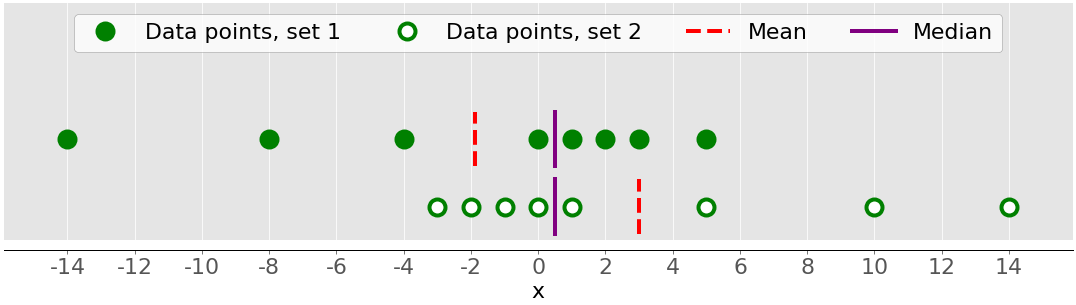
The primary set is represented by the inexperienced dots and the second with the white ones. Often, unfavorable skewness values point out that there’s a dominant tail on the left facet, which you’ll see with the primary set. Constructive skewness values correspond to an extended or fatter tail on the fitting facet, which you’ll see within the second set. If the skewness is near 0 (for instance, between −0.5 and 0.5), then the dataset is taken into account fairly symmetrical.
When you’ve calculated the dimensions of your dataset n, the pattern imply mean_, and the usual deviation std_, you will get the pattern skewness with pure Python:
The skewness is constructive, so x has a right-side tail.
You can even calculate the pattern skewness with scipy.stats.skew():
The obtained end result is identical because the pure Python implementation. The parameter bias is ready to False to allow the corrections for statistical bias. The non-obligatory parameter nan_policy can take the values "propagate", "elevate", or "omit". It lets you management the way you’ll deal with nan values.
pandas Sequence objects have the strategy .skew() that additionally returns the skewness of a dataset:
Like different strategies, .skew() ignores nan values by default, due to the default worth of the non-obligatory parameter skipna.
Percentiles
The pattern 𝑝 percentile is the aspect within the dataset such that 𝑝% of the weather within the dataset are lower than or equal to that worth. Additionally, (100 − 𝑝)% of the weather are better than or equal to that worth. If there are two such parts within the dataset, then the pattern 𝑝 percentile is their arithmetic imply. Every dataset has three quartiles, that are the percentiles that divide the dataset into 4 components:
- The primary quartile is the pattern twenty fifth percentile. It divides roughly 25% of the smallest objects from the remainder of the dataset.
- The second quartile is the pattern fiftieth percentile or the median. Roughly 25% of the objects lie between the primary and second quartiles and one other 25% between the second and third quartiles.
- The third quartile is the pattern seventy fifth percentile. It divides roughly 25% of the biggest objects from the remainder of the dataset.
Every half has roughly the identical variety of objects. If you wish to divide your information into a number of intervals, then you should utilize statistics.quantiles():
On this instance, 8.0 is the median of x, whereas 0.1 and 21.0 are the pattern twenty fifth and seventy fifth percentiles, respectively. The parameter n defines the variety of ensuing equal-probability percentiles, and technique determines how one can calculate them.
Observe: statistics.quantiles() is launched in Python 3.8.
You can even use np.percentile() to find out any pattern percentile in your dataset. For instance, that is how yow will discover the fifth and ninety fifth percentiles:
percentile() takes a number of arguments. You must present the dataset as the primary argument and the percentile worth because the second. The dataset could be within the type of a NumPy array, listing, tuple, or comparable information construction. The percentile could be a quantity between 0 and 100 like within the instance above, nevertheless it will also be a sequence of numbers:
This code calculates the twenty fifth, fiftieth, and seventy fifth percentiles . If the percentile worth is a sequence, then percentile() returns a NumPy array with the outcomes. The primary assertion returns the array of quartiles. The second assertion returns the median, so you’ll be able to verify it’s equal to the fiftieth percentile, which is 8.0.
If you wish to ignore nan values, then use np.nanpercentile() as an alternative:
That’s how one can keep away from nan values.
NumPy additionally gives you very comparable performance in quantile() and nanquantile(). When you use them, then you definitely’ll want to offer the quantile values because the numbers between 0 and 1 as an alternative of percentiles:
The outcomes are the identical as within the earlier examples, however right here your arguments are between 0 and 1. In different phrases, you handed 0.05 as an alternative of 5 and 0.95 as an alternative of 95.
pd.Sequence objects have the strategy .quantile():
.quantile() additionally wants you to offer the quantile worth because the argument. This worth could be a quantity between 0 and 1 or a sequence of numbers. Within the first case, .quantile() returns a scalar. Within the second case, it returns a brand new Sequence holding the outcomes.
Ranges
The vary of knowledge is the distinction between the utmost and minimal aspect within the dataset. You may get it with the perform np.ptp():
This perform returns nan if there are nan values in your information, whether or not you cross a NumPy array or a pandas Sequence.
Alternatively, you should utilize built-in Python, NumPy, or pandas features and strategies to calculate the maxima and minima of sequences:
Listed here are some examples of how you’d use these routines:
That’s the way you get the vary of knowledge.
The interquartile vary is the distinction between the primary and third quartile. When you calculate the quartiles, you’ll be able to take their distinction:
Observe that you simply entry the values in a pandas Sequence object with the labels 0.75 and 0.25.
Abstract of Descriptive Statistics
SciPy and pandas supply helpful routines to shortly get descriptive statistics with a single perform or technique name. You should utilize scipy.stats.describe() like this:
You must present the dataset as the primary argument. The argument could be a NumPy array, listing, tuple, or comparable information construction. You’ll be able to omit ddof=1 because it’s the default and solely issues if you’re calculating the variance. You’ll be able to cross bias=False to pressure correcting the skewness and kurtosis for statistical bias.
Observe: The non-obligatory parameter nan_policy can take the values "propagate" (default), "elevate" (an error), or "omit". This parameter lets you management what’s occurring when there are nan values.
describe() returns an object that holds the next descriptive statistics:
nobs: the variety of observations or parts in your datasetminmax: the tuple with the minimal and most values of your datasetimply: the imply of your datasetvariance: the variance of your datasetskewness: the skewness of your datasetkurtosis: the kurtosis of your dataset
You’ll be able to entry explicit values with dot notation:
With SciPy, you’re only one perform name away from a descriptive statistics abstract on your dataset.
pandas has comparable, if not higher, performance. Sequence objects have the strategy .describe():
It returns a brand new Sequence that holds the next:
rely: the variety of parts in your datasetimply: the imply of your datasetstd: the usual deviation of your datasetminandmax: the minimal and most values of your dataset25%,50%, and75%: the quartiles of your dataset
If you would like the ensuing Sequence object to include different percentiles, then it is best to specify the worth of the non-obligatory parameter percentiles. You’ll be able to entry every merchandise of end result with its label:
That’s how one can get descriptive statistics of a Sequence object with a single technique name utilizing pandas.
Measures of Correlation Between Pairs of Information
You’ll usually want to look at the connection between the corresponding parts of two variables in a dataset. Say there are two variables, 𝑥 and 𝑦, with an equal variety of parts, 𝑛. Let 𝑥₁ from 𝑥 correspond to 𝑦₁ from 𝑦, 𝑥₂ from 𝑥 to 𝑦₂ from 𝑦, and so forth. You’ll be able to then say that there are 𝑛 pairs of corresponding parts: (𝑥₁, 𝑦₁), (𝑥₂, 𝑦₂), and so forth.
You’ll see the next measures of correlation between pairs of knowledge:
- Constructive correlation exists when bigger values of 𝑥 correspond to bigger values of 𝑦 and vice versa.
- Adverse correlation exists when bigger values of 𝑥 correspond to smaller values of 𝑦 and vice versa.
- Weak or no correlation exists if there isn’t a such obvious relationship.
The next determine exhibits examples of unfavorable, weak, and constructive correlation:
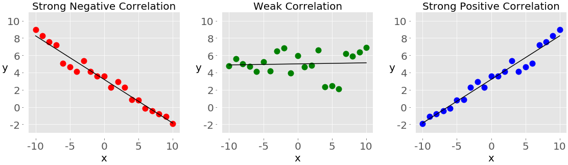
The plot on the left with the purple dots exhibits unfavorable correlation. The plot within the center with the inexperienced dots exhibits weak correlation. Lastly, the plot on the fitting with the blue dots exhibits constructive correlation.
Observe: There’s one vital factor it is best to at all times take into consideration when working with correlation amongst a pair of variables, and that’s that correlation just isn’t a measure or indicator of causation, however solely of affiliation!
The 2 statistics that measure the correlation between datasets are covariance and the correlation coefficient. Let’s outline some information to work with these measures. You’ll create two Python lists and use them to get corresponding NumPy arrays and pandas Sequence:
Now that you’ve got the 2 variables, you can begin exploring the connection between them.
Covariance
The pattern covariance is a measure that quantifies the energy and course of a relationship between a pair of variables:
- If the correlation is constructive, then the covariance is constructive, as nicely. A stronger relationship corresponds to the next worth of the covariance.
- If the correlation is unfavorable, then the covariance is unfavorable, as nicely. A stronger relationship corresponds to a decrease (or greater absolute) worth of the covariance.
- If the correlation is weak, then the covariance is near zero.
The covariance of the variables 𝑥 and 𝑦 is mathematically outlined as 𝑠ˣʸ = Σᵢ (𝑥ᵢ − imply(𝑥)) (𝑦ᵢ − imply(𝑦)) / (𝑛 − 1). Right here, 𝑖 = 1, 2, …, 𝑛, whereas imply(𝑥) and imply(𝑦) are the pattern technique of 𝑥 and 𝑦. It follows that the covariance of two similar variables is definitely the variance: 𝑠ˣˣ = Σᵢ(𝑥ᵢ − imply(𝑥))² / (𝑛 − 1) = (𝑠ˣ)² and 𝑠ʸʸ = Σᵢ(𝑦ᵢ − imply(𝑦))² / (𝑛 − 1) = (𝑠ʸ)².
That is how one can calculate the covariance in pure Python:
First, it’s important to discover the imply of x and y. Then, you apply the mathematical system for the covariance.
NumPy has the perform cov() that returns the covariance matrix:
Observe that cov() has the non-obligatory parameters bias, which defaults to False, and ddof, which defaults to None. Their default values are appropriate for getting the pattern covariance matrix. The upper-left aspect of the covariance matrix is the covariance of x and x, or the variance of x. Equally, the lower-right aspect is the covariance of y and y, or the variance of y. You’ll be able to test to see that that is true:
As you’ll be able to see, the variances of x and y are equal to cov_matrix[0, 0] and cov_matrix[1, 1], respectively.
The opposite two parts of the covariance matrix are equal and signify the precise covariance between x and y:
You’ve obtained the identical worth of the covariance with np.cov() as with pure Python.
pandas Sequence have the strategy .cov() that you should utilize to calculate the covariance:
Right here, you name .cov() on one Sequence object and cross the opposite object as the primary argument.
Correlation Coefficient
The correlation coefficient, or Pearson product-moment correlation coefficient, is denoted by the image 𝑟. The coefficient is one other measure of the correlation between information. You’ll be able to consider it as a standardized covariance. Listed here are some vital info about it:
- The worth 𝑟 > 0 signifies constructive correlation.
- The worth 𝑟 < 0 signifies unfavorable correlation.
- The worth r = 1 is the utmost doable worth of 𝑟. It corresponds to an ideal constructive linear relationship between variables.
- The worth r = −1 is the minimal doable worth of 𝑟. It corresponds to an ideal unfavorable linear relationship between variables.
- The worth r ≈ 0, or when 𝑟 is round zero, implies that the correlation between variables is weak.
The mathematical system for the correlation coefficient is 𝑟 = 𝑠ˣʸ / (𝑠ˣ𝑠ʸ) the place 𝑠ˣ and 𝑠ʸ are the usual deviations of 𝑥 and 𝑦 respectively. When you’ve got the means (mean_x and mean_y) and commonplace deviations (std_x, std_y) for the datasets x and y, in addition to their covariance cov_xy, then you’ll be able to calculate the correlation coefficient with pure Python:
You’ve received the variable r that represents the correlation coefficient.
scipy.stats has the routine pearsonr() that calculates the correlation coefficient and the 𝑝-value:
pearsonr() returns a tuple with two numbers. The primary one is 𝑟 and the second is the 𝑝-value.
Much like the case of the covariance matrix, you’ll be able to apply np.corrcoef() with x_ and y_ because the arguments and get the correlation coefficient matrix:
The upper-left aspect is the correlation coefficient between x_ and x_. The lower-right aspect is the correlation coefficient between y_ and y_. Their values are equal to 1.0. The opposite two parts are equal and signify the precise correlation coefficient between x_ and y_:
In fact, the end result is identical as with pure Python and pearsonr().
You may get the correlation coefficient with scipy.stats.linregress():
linregress() takes x_ and y_, performs linear regression, and returns the outcomes. slope and intercept outline the equation of the regression line, whereas rvalue is the correlation coefficient. To entry explicit values from the results of linregress(), together with the correlation coefficient, use dot notation:
That’s how one can carry out linear regression and acquire the correlation coefficient.
pandas Sequence have the strategy .corr() for calculating the correlation coefficient:
It is best to name .corr() on one Sequence object and cross the opposite object as the primary argument.

