Steer Beams to Actuality: from Phased Array to Beamforming » Scholar Lounge

In immediately’s submit, Liping from the Scholar Packages Staff will share her expertise on how MATLAB and Simulink may help college students to know wi-fi communication theories on beamforming and precoding. Allow us to see what she goes to share.

Once I took the course “Fundamentals of Wi-fi Communications”, I felt it was so laborious to pay attention within the courses because the course materials was stuffed with arithmetic together with matrices, stochastic processes, formulation derivations, and so forth. After engaged on wi-fi communication techniques corresponding to LTE and 5G for a few years, I discovered understanding the essential ideas and theories was so vital since they’re elementary to completely different functions.

Many examples and reference functions in MATLAB may help you to know complicated wi-fi communication theories. On this script, I’ll present how a demo may help you to know beamforming, a method that has been broadly utilized in 5G and even in 6G, radar, sonar, medical imaging, and audio array techniques.

What are Phased Arrays?

In wi-fi communications, the weather of a phased array may very well be antennas. From the snapshots beneath of Douglas’ video, you’ll be able to see in the proper determine that the beams of a Uniform Linear Array (ULA) of isotropic antennas, the place indicators from every antenna have been superimposed so the sign power has been enhanced in some instructions, whereas they’ve been canceled within the different instructions.

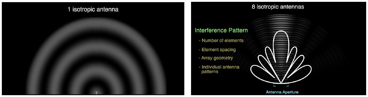
The beam sample of an antenna array is dependent upon the settings together with the variety of antenna parts, spacing between parts, array geometry in addition to particular person antenna patterns.

When wanting by means of the next instance on the best way to use the Sensor Array Analyzer, you discover the App may help with tuning parameters, visualizing the beam sample of a phased array, in addition to steering a phased array to a sure path. With completely different steering vectors, you’ll be able to transfer beams round with out transferring the array bodily.

Now you should still be interested by the best way to use beam steering to enhance the efficiency of a wi-fi communication system. The reply is by beamforming, a scheme to pre-steer beams to a desired path! The subsequent instance will present you the best way to do beamforming of an antenna array to enhance the Sign-to-Noise Ratio (SNR) of a wi-fi hyperlink.

Easy methods to do Beamforming?

Antenna arrays have develop into a part of the usual configuration in 5G. Such wi-fi communication techniques are also known as A number of-Enter-and-A number of-Output (MIMO) techniques. To indicate the benefits of a number of antennas, we assume a wi-fi hyperlink deployed at 60 GHz, a millimeter wave frequency that had been newly thought of in 5G.

With no loss in generality, we place a transmitter on the origin and a receiver roughly 1.6 km away.

Then the Angle of Departure (AoD) and the Angle of Arrival (AoA) could be calculated based mostly on the middle places of the transmitter and the receiver.

Subsequent, we contemplate two representive channel varieties.

Line-of-Sight Channel

Line-of-Sight (LOS) propagation is the best wi-fi channel that usually occurred in rural areas. Does adopting an antenna array beneath LOS propagation can improve the SNR on the receiver and thus enhance the hyperlink’s bit error fee (BER)?

As a benchmark, you would simulate the BER efficiency of a Single-Enter-and-Single-output (SISO) hyperlink beneath a LOS channel as follows, the place the scatteringchanmtx operate is used to create a channel matrix for various transmit and obtain array configurations. The operate simulates a number of scatterers between the transmit and the obtain arrays assuming the sign travels from the transmit array to all of the scatterers first after which bounces off the scatterers and arrives on the obtain array. On this case, every scatterer defines a sign path between the transmit and the obtain array, so the ensuing channel matrix describes a multipath atmosphere. You may learn the main points of this operate by deciding on it after which right-clicking to open the operate.

Take into account a SISO communication hyperlink the place each the transmitter and the receiver solely have a single antenna positioned on the node middle, and there’s a direct path from the transmitter to the receiver. Such a LOS channel could be modeled as a particular case of a multipath atmosphere.

You’ve got the BER efficiency of a SISO LOS hyperlink. When wanting into the main points of the helperMIMOBER operate given within the Helper Capabilities session on the finish of this script, it’s best to discover BPSK modulation is taken into account in all of the instances.

Now contemplate a MIMO hyperlink. we assume each the transmitter and the receiver are 4-element ULAs with half-wavelength spacing,

With the obtain antenna array, the obtained indicators throughout array parts of the receiver are coherent, so it’s doable to pre-steer the obtain array towards the transmitter to enhance the SNR. Furthermore, the transmitter can also pre-steer the principle beam of its antenna array towards the receiver for additional enchancment.

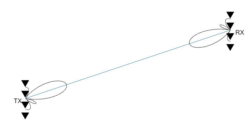
With beamforming, the modulated sign must be multiplied with wt earlier than sending out on the transmitter, whereas the obtained sign must be multiplied with wr earlier than demodulation on the receiver. After utilizing the helperPlotSpatialMIMOScene operate to visualise the scene within the determine above, you discover the principle beams on the transmitter and the receiver have been pointed at one another.

Now you’ll be able to examine the BER efficiency within the SISO and the MIMO instances beneath the LOS propagation channel,

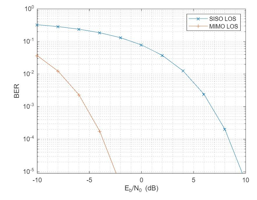
The BER curve exhibits the transmit array and the obtain array contribute round 6 dB array acquire respectively, leading to a complete acquire of 12 dB over the SISO case.

Observe that the acquire is achieved beneath the belief that the transmitter must know the receiver’s path or location, and in the meantime the sign incoming path is thought to the receiver, the place the angle is usually obtained utilizing the path of arrival estimation algorithms.

Multipath Channel

Typically, wi-fi communications happen in a multipath fading atmosphere. The remainder of this instance explores how phased arrays may help in such a case.

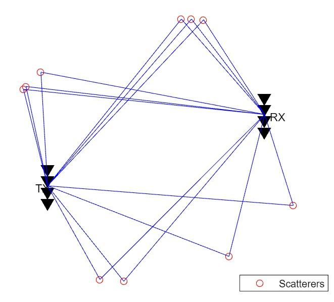
Assume there are 10 randomly positioned scatterers within the channel, so there will probably be 10 paths from the transmitter to the receiver, as illustrated within the following.

For simplicity, assume that indicators touring alongside all paths arrive throughout the identical image interval, so the channel is frequency flat and never frequency selective.

In such a multipath fading channel, the channel wants to alter over a number of time slots to simulate the BER curve. Assume the simulation lasts 1000 frames and every body has 10000 bits. The BER curve of the baseline SISO hyperlink beneath a multipath channel could be simulated as follows.

In SISO instances, should you examine the channel matrix of a LOS channel with that of a multipath channel, you’ll be able to discover it incorporates a single ingredient and the worth of the ingredient adjustments from an actual quantity to a posh quantity resulting from multipath fading. In such a case, a combining weight calculated as wr = sisompchan’/norm(sisompchan) can be utilized on the receiver to enhance the SNR.

Within the MIMO case, the BER curve could be simulated as follows, the place the diagbfweights operate is used to calculate the precoding weight wp on the transmitter and the combining weights wc on the receiver. You may right-click on the operate and open it to see its particulars.

To grasp how precoding and mixing weights are calculated, you first want to know what Singular Worth Decomposition (SVD) is. Use the next command to seek out the MATLAB documentation on SVD.

Briefly, an SVD ([U,S,V] = svd(X)) produces a diagonal matrix S, of the identical dimension as X and with nonnegative diagonal parts in reducing order, and unitary matrices U and V in order that X = U*S*V’. Attempt following instructions in MATLAB.

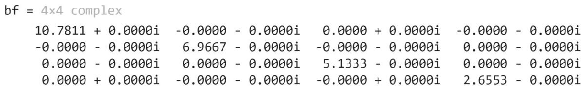
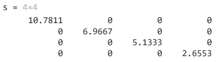
Evaluate bf with s, you now know the diagbfweights operate is predicated on SVD. Because of a wealthy scatterer atmosphere, the channel matrix of a MIMO multipath channel normally has full rank.

Observe that the product wp*mimompchan*wc is a diagonal matrix, which signifies that the knowledge obtained by every obtain array ingredient is just a scaled model of the transmit array ingredient. Such a MIMO multipath channel behaves like a number of orthogonal subchannels throughout the authentic channel.

Due to this fact, it’s doable to ship a number of information streams concurrently throughout the MIMO multipath channel, which known as spatial multiplexing. The fundamental concept of spatial multiplexing is to separate the channel matrix into a number of modes in order that the info stream despatched from completely different parts within the transmit array could be independently recovered from the obtained sign. The aim of spatial multiplexing is much less about rising the SNR and extra about rising the knowledge throughput.

Now you’ll be able to plot the BER curves of the SISO multipath case, and the primary two information streams within the MIMO multipath case. As a benchmark, you additionally plot the BER curve within the SISO LOS case that has been received from the earlier part.

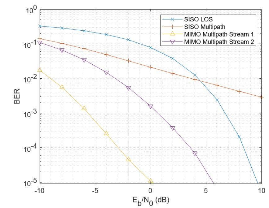
In comparison with the BER curve of the SISO LOS channel, the BER curve of the SISO multipath channel falls off a lot slower as a result of fading brought on by the multipath propagation. In the meantime, within the MIMO multipath case, the primary subchannel corresponds to the dominant transmit and obtain instructions so there isn’t a loss within the range acquire, which refers back to the acquire on the slope change. Though the second stream can’t present a acquire as excessive as the primary stream because it makes use of a much less dominant subchannel, the general data throughput could be improved since it’s now doable to transmit a number of information streams concurrently.

Abstract

This demo explains how array processing can enhance the efficiency of a MIMO wi-fi communication system. Relying on the character of the channel, the arrays can be utilized to both enhance the SNR through array acquire or range acquire; or enhance the capability through spatial multiplexing.

Additional Exploration

Helper Capabilities

The primary helper operate is for plotting the MIMO scene in a 2D space.

The second helper operate is for calculating the BER values of a MIMO hyperlink.

Within the first two capabilities, a SISO scene/hyperlink could be thought of as a particular case of a MIMO scene/hyperlink.

The third operate is for calculating the place of the scatterers.

The fourth operate is for plotting BER curves.