


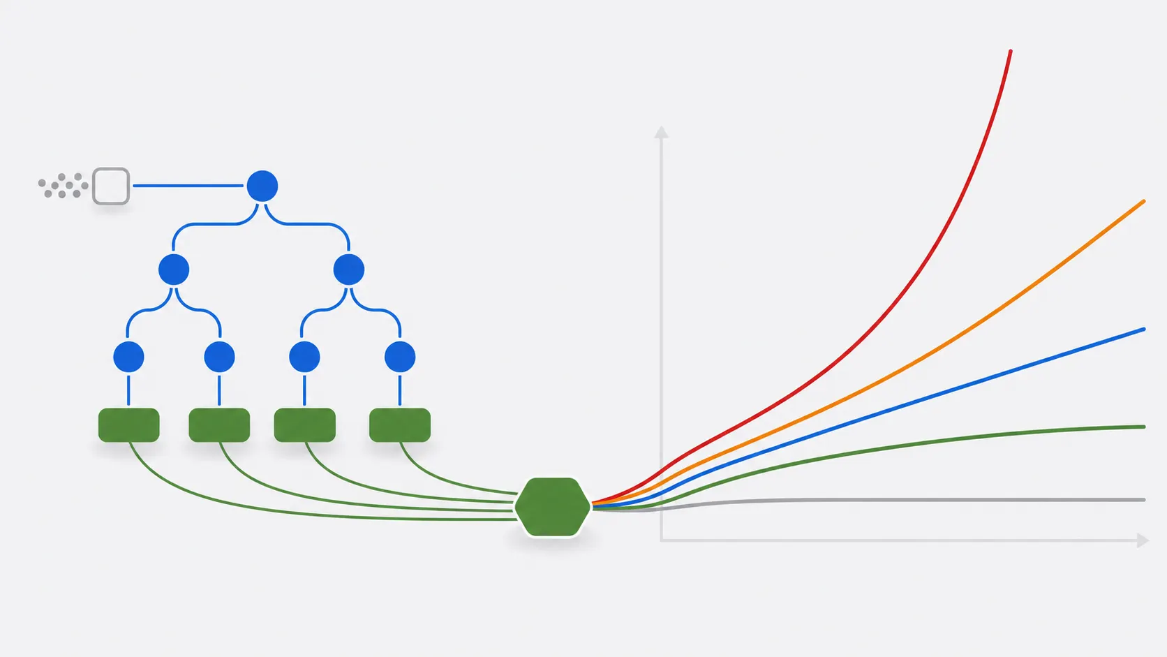
At an enter dimension of 1 million, an O(log n) algorithm takes about 20 steps. An O(n²) algorithm takes a trillion. No quantity of quicker {hardware}, tighter loops or higher compiler flags closes that hole — solely selecting a distinct algorithm does.
That’s the reason this record exists, and why each entry under carries its complexity alongside the outline. These are ten algorithm households quite than ten particular person algorithms, as a result of that’s how the data is definitely helpful: you not often have to recall Dijkstra’s actual steps, however you do have to recognise a shortest-path downside when one arrives disguised as a enterprise requirement.
Desk of Contents
Complexity at a Look
| Household | Typical time | House | Use when |
|---|---|---|---|
| Sorting (comparability) | O(n log n) | O(1)–O(n) | Information have to be ordered, or ordering permits a quicker subsequent step |
| Binary search | O(log n) | O(1) | Information is already sorted and also you want lookups |
| Hashing | O(1) common | O(n) | You want quick lookup by key and order doesn’t matter |
| Graph traversal (BFS/DFS) | O(V + E) | O(V) | Exploring connections, reachability, shortest unweighted path |
| Shortest path (Dijkstra) | O((V + E) log V) | O(V) | Weighted graph, non-negative edges |
| Minimal spanning tree | O(E log E) | O(V) | Join every part at minimal complete value |
| Dynamic programming | Downside-specific | O(n)–O(n²) | Overlapping subproblems with optimum substructure |
| Divide and conquer | Typically O(n log n) | O(log n) stack | The issue splits cleanly into unbiased halves |
| Backtracking | Typically exponential | O(depth) | Constraint satisfaction with a searchable resolution house |
| String matching (KMP) | O(n + m) | O(m) | Repeated sample search in massive textual content |
Two issues this desk is just not. It isn’t an alternative choice to measuring — constants matter, and an O(n²) algorithm on 50 components will beat an O(n log n) one with a heavy fixed issue. And common case is just not worst case: hashing is O(1) till each key collides, and quicksort is O(n log n) till the pivot selection degenerates.
1. Sorting Algorithms
Sorting is the most-implemented household within the record, and the one most frequently reached for unnecessarily — a lot of its worth is as a preprocessing step that makes one thing else quick. Sorted information permits binary search, makes duplicate detection linear, and turns many vary queries into two lookups.
Know these three: quicksort (quick in follow, O(n log n) common, O(n²) worst), merge type (assured O(n log n), secure, wants O(n) further house), and one easy quadratic type resembling insertion type so that you perceive what the environment friendly ones enhance upon.
In manufacturing, name the library type. std::type, Arrays.type and sorted() have absorbed many years of edge circumstances — introsort switches to heapsort when quicksort’s recursion runs too deep, and Timsort exploits the partial ordering actual information normally has.
On-site implementations: the quicksort information covers Lomuto versus Hoare partitioning with measured swap counts and code in 5 languages, and shell type exhibits the gap-sequence concept that bridges insertion type and the O(n log n) household.
2. Search Algorithms
Binary search is the one to internalise: O(log n) on sorted information, and the supply of an unreasonable variety of off-by-one bugs. Jon Bentley’s commentary that almost all programmers can not write it accurately on the primary try has held up remarkably nicely.
Linear search is O(n) and is genuinely the best reply for small or unsorted collections — the price of sorting first is just price paying if you’ll search repeatedly.
The choice rule: search as soon as on unsorted information, use linear. Search repeatedly, type as soon as then binary search, or construct a hash desk.
3. Hashing
Hashing trades reminiscence for velocity, changing a key into an array index so lookup is O(1) on common quite than O(log n) or O(n). It’s the mechanism behind std::unordered_map, Python’s dict, Java’s HashMap, and hash indexes in database programs.
What to really perceive: collisions are inevitable — the pigeonhole precept ensures it — so the attention-grabbing half is how they’re resolved (chaining versus open addressing), and what occurs to that O(1) assure when the load issue climbs or an adversary chooses colliding keys intentionally.
Cryptographic hashes resembling SHA-256 resolve a distinct downside — integrity and irreversibility quite than quick lookup — and the 2 shouldn’t be conflated.
4. Graph Traversal: BFS and DFS
Many foundational graph issues begin with considered one of these two traversals.
Breadth-first search explores degree by degree utilizing a queue, and finds the shortest path in an unweighted graph as a facet impact. Depth-first search follows one path to exhaustion utilizing a stack or recursion, and is the idea for cycle detection, topological sorting and linked parts.
Each are O(V + E). The selection is about form: BFS once you need the closest factor, DFS once you need to know whether or not a path exists in any respect or have to discover exhaustively.
5. Shortest Path: Dijkstra and Pals
Dijkstra’s algorithm finds the shortest path in a weighted graph with non-negative edges, in O((V + E) log V) with a binary heap. It’s a basis for route-planning algorithms and is utilized in link-state routing resembling OSPF, in addition to many different weighted-graph issues.
The constraint that catches folks out: non-negative edges solely. With unfavourable weights, Dijkstra’s grasping selection stops being secure and also you want Bellman-Ford (O(V·E), slower however tolerates unfavourable edges and detects unfavourable cycles).
6. Minimal Spanning Bushes
Given a weighted graph, join each vertex on the lowest complete value. That is community design in its purest type — laying cable, planning pipelines, or clustering.
Kruskal’s algorithm types each edge and greedily accepts any that doesn’t create a cycle, utilizing union-find for the cycle verify. Prim’s algorithm grows a single tree outward from a begin vertex. Each are grasping, each are right, and the selection is about enter form: Kruskal for sparse graphs with an edge record, Prim for dense graphs with an adjacency construction.
On-site implementation: the Kruskal’s algorithm information covers union-find with path compression and union by rank, with a step-by-step hint and code in C and C++.
7. Dynamic Programming
The household that almost all reliably separates individuals who have practised from individuals who haven’t.
Dynamic programming applies when an issue has overlapping subproblems and optimum substructure — the identical smaller issues recur, and an optimum general reply is constructed from optimum partial solutions. The approach is to resolve every subproblem as soon as and retailer the outcome, both top-down with memoisation or bottom-up with a desk.
Naive recursive Fibonacci is O(2ⁿ); memoised, it’s O(n). That single instance is the entire concept, and it’s price implementing each to really feel the distinction.
On-site implementation: the knapsack downside is the canonical DP train — maximise worth below a weight constraint — and it generalises to useful resource allocation, budgeting and scheduling.
8. Divide and Conquer
Break up the issue into unbiased subproblems, resolve them recursively, mix the outcomes. Merge type, quicksort, binary search and the quick Fourier rework all observe this form.
It’s price distinguishing from dynamic programming, for the reason that two are often confused: divide and conquer subproblems are unbiased; dynamic programming subproblems overlap. That distinction is precisely why DP wants a memo desk and divide and conquer doesn’t.
9. Backtracking
Discover candidate options incrementally and abandon a department as quickly because it can not result in a legitimate reply. N-Queens, Sudoku solvers, maze pathfinding and constraint satisfaction all sit right here.
Backtracking is often exponential within the worst case, however pruning — recognising a lifeless department early — is what makes it sensible. The hole between a naive implementation and a well-pruned one is usually the distinction between seconds and centuries.
10. String Matching
Discovering a sample inside a bigger textual content. The naive method is O(n·m); Knuth-Morris-Pratt achieves O(n + m) by precomputing how far it could actually safely skip after a mismatch, and Rabin-Karp makes use of a rolling hash, which makes it the pure selection for looking out a number of patterns without delay.
Most languages offer you this in the usual library — std::string::discover, str.index, String.indexOf — and for something involving real sample languages quite than fastened substrings, a daily expression engine has already solved it higher than you’ll.
Easy methods to Truly Be taught These
Studying about algorithms produces recognition, not recall. The hole closes solely by implementation.
- Implement each as soon as from scratch, with out a reference. The bugs you hit are the educational.
- Then learn a great implementation and be aware what it does in another way — normally edge circumstances and constant-factor work you didn’t take into consideration.
- Practise recognising them in disguise. Interview questions and actual necessities not often say “use Dijkstra”; they are saying “discover the most cost effective route”. Aggressive programming websites are the quickest option to construct that recognition.
- Be taught the complexity, not the code. In six months you’ll not bear in mind KMP’s failure-function development. It’s best to do not forget that repeated substring search has an O(n + m) resolution, which is sufficient to discover it once more.
For algorithm-focused interviews: these households above cowl the overwhelming majority of questions requested. Depth on sorting, binary search, hashing, BFS/DFS and dynamic programming is price greater than shallow familiarity with all ten.
Key Takeaways
- Complexity dominates optimisation. At n = 1,000,000, O(log n) is ~20 steps and O(n²) is 10¹². No micro-optimisation crosses that hole.
- Be taught households, not situations. Recognising a shortest-path downside issues greater than recalling Dijkstra’s pseudocode.
- Common case is just not worst case. Hashing is O(1) till it collides; quicksort is O(n log n) till the pivot degenerates.
- Divide and conquer has unbiased subproblems; dynamic programming has overlapping ones. That single distinction explains why one wants a memo desk.
- Dijkstra requires non-negative edges. Adverse weights want Bellman-Ford.
- Use the library implementation in manufacturing and write your personal solely to study.
Often Requested Questions
Conclusion
The rationale this record is ten households quite than ten algorithms is that the recall you want in follow is just not procedural. No person writes Dijkstra’s from reminiscence at work; they recognise that an issue is a weighted shortest path, search for the main points, and know roughly what it’s going to value to run. That recognition is the transferable ability, and it’s constructed by implementing issues as soon as quite than studying about them repeatedly.
The complexity desk is the half price preserving shut. Most efficiency issues in actual programs aren’t sluggish code — they’re the best code utilized at a scale it was by no means chosen for, and the repair is a distinct algorithm quite than a quicker loop. The algorithms part covers particular person implementations in depth as you’re employed by them.

