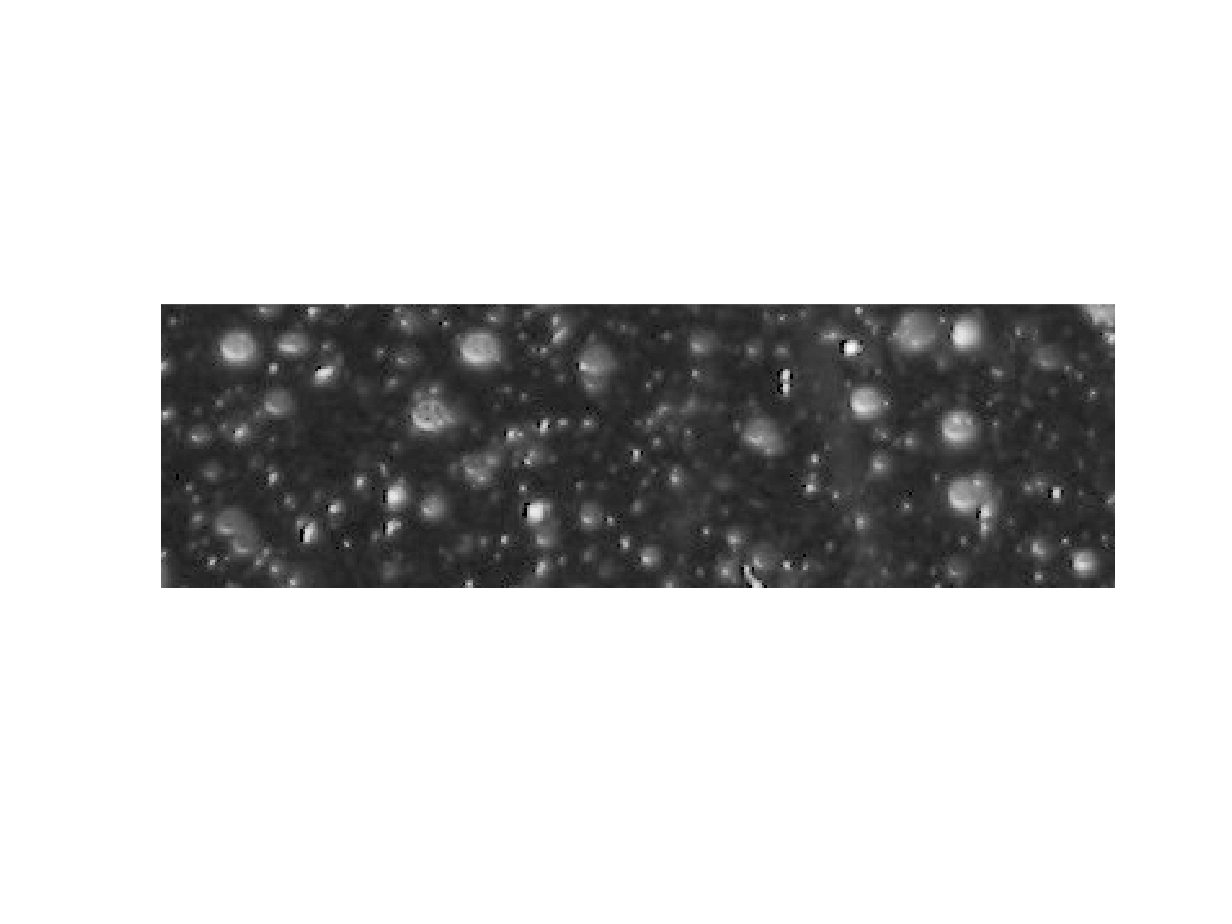
url = “https://blogs.mathworks.com/steve/information/snowflakes2.png”;
imshow(A)
I would wish to see if we are able to focus algorithmically on these white blobby issues (that is a technical time period that I discovered in engineering college). First, let’s attempt computing the regional maxima.
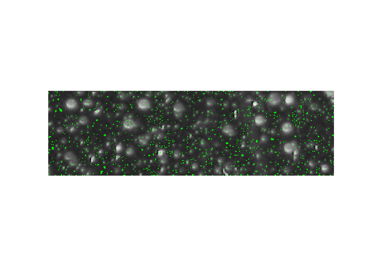
A_regmax = imregionalmax(A);
imshow(A_regmax)

At first look, that does not seem like what I am after. Let’s discover out what is going on on right here.
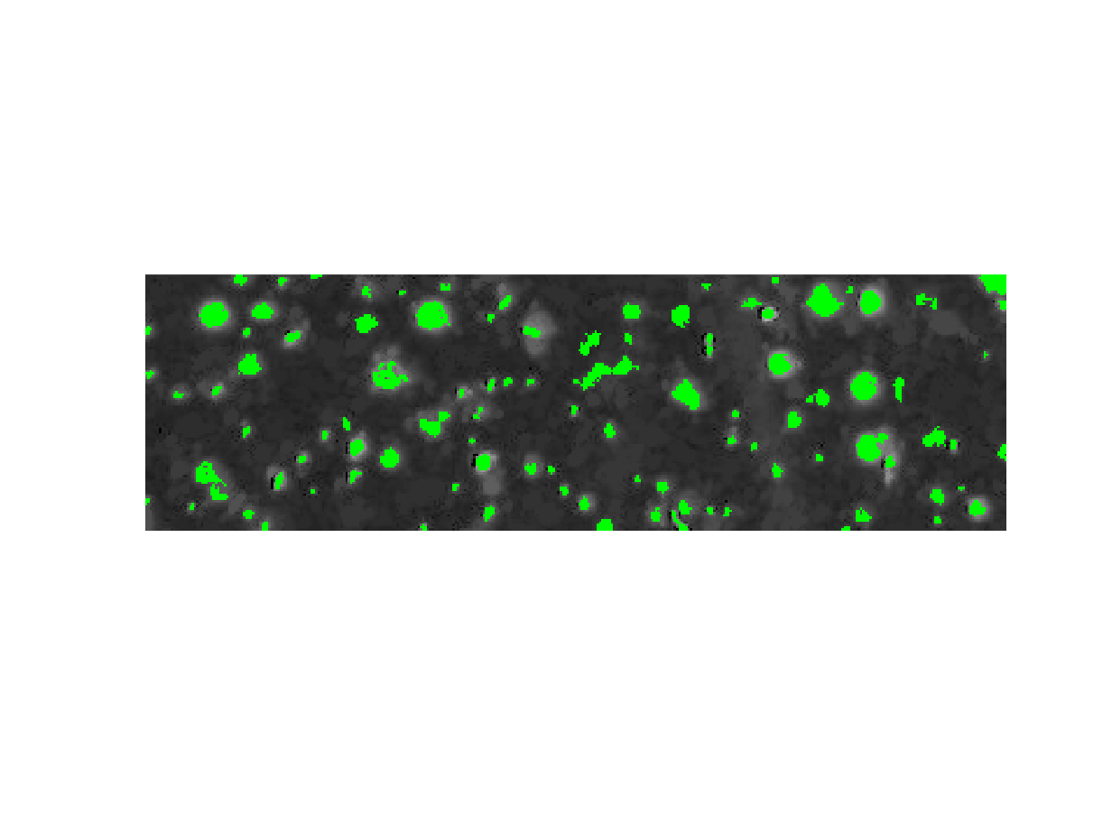
A_regmax_overlay = imoverlay(A,A_regmax,“inexperienced”);
imshow(A_regmax_overlay)
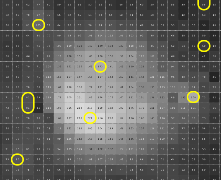
I need to look carefully at one white blobby factor specifically.
imshow(A_regmax_overlay(30:47,263:285,:))
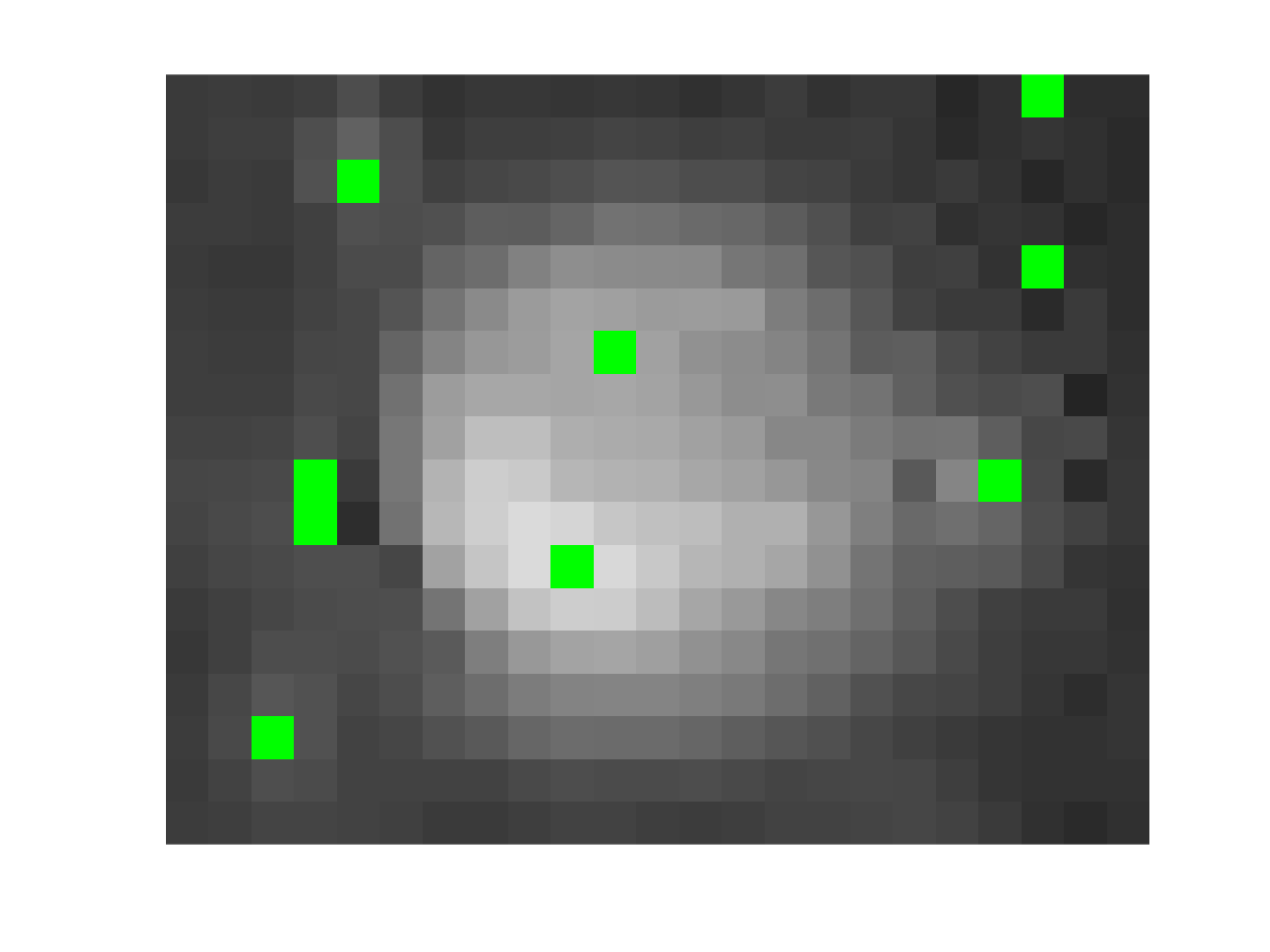
One, or possibly two, of those areas seems just like the form of peak that we’re taken with. What in regards to the others? Let me present you two other ways to discover additional. The primary is with a 3-D visualization, the place we deal with the picture pixel values as heights of a grey floor. The code under reveals that floor, after which it shows the detected regional maxima as blue-and-yellow dots simply above the floor.
A_cropped = A(30:47,263:285);
A_regmax_cropped = A_regmax(30:47,263:285);
surf(A_cropped, EdgeColor = “none”)
[y,x,~] = discover(A_regmax_cropped);
z = A_cropped(A_regmax_cropped);
plot3(x,y,z+1,LineStyle=“none”,Marker=“o”,…
set(gca,YDir = “reverse”)
maintain off

With both approach, you will get the concept a number of of those maxima areas are simply small, uninteresting fluctuations.
As I mentioned within the earlier posts, you should use the h-maxima rework to filter out these small peaks.
imshow(B(30:47,263:285))
B_regmax = imregionalmax(B);
imshow(B_regmax(30:47,263:285))

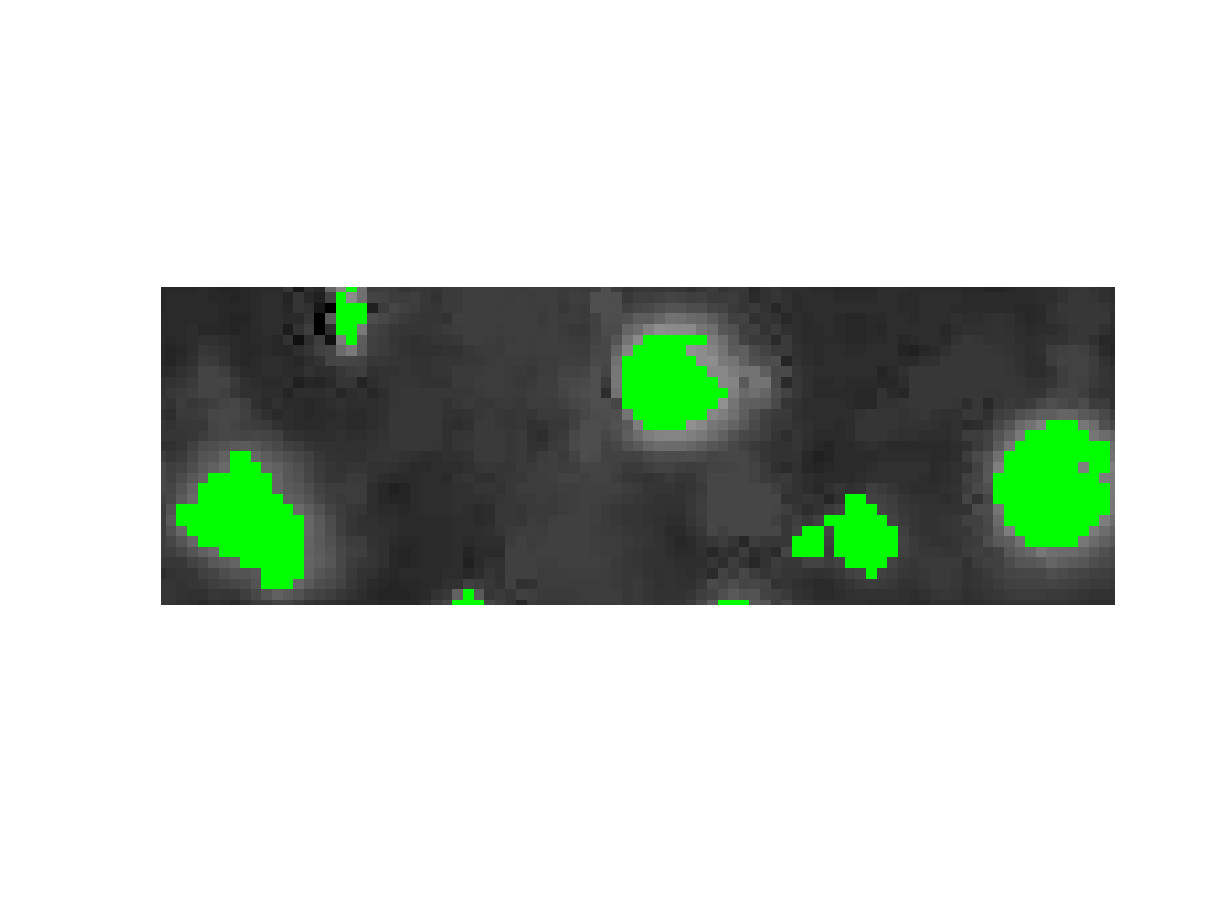
B_regmax_overlay = imoverlay(B,B_regmax,“inexperienced”);
imshow(B_regmax_overlay)
axis([225 315 30 60])
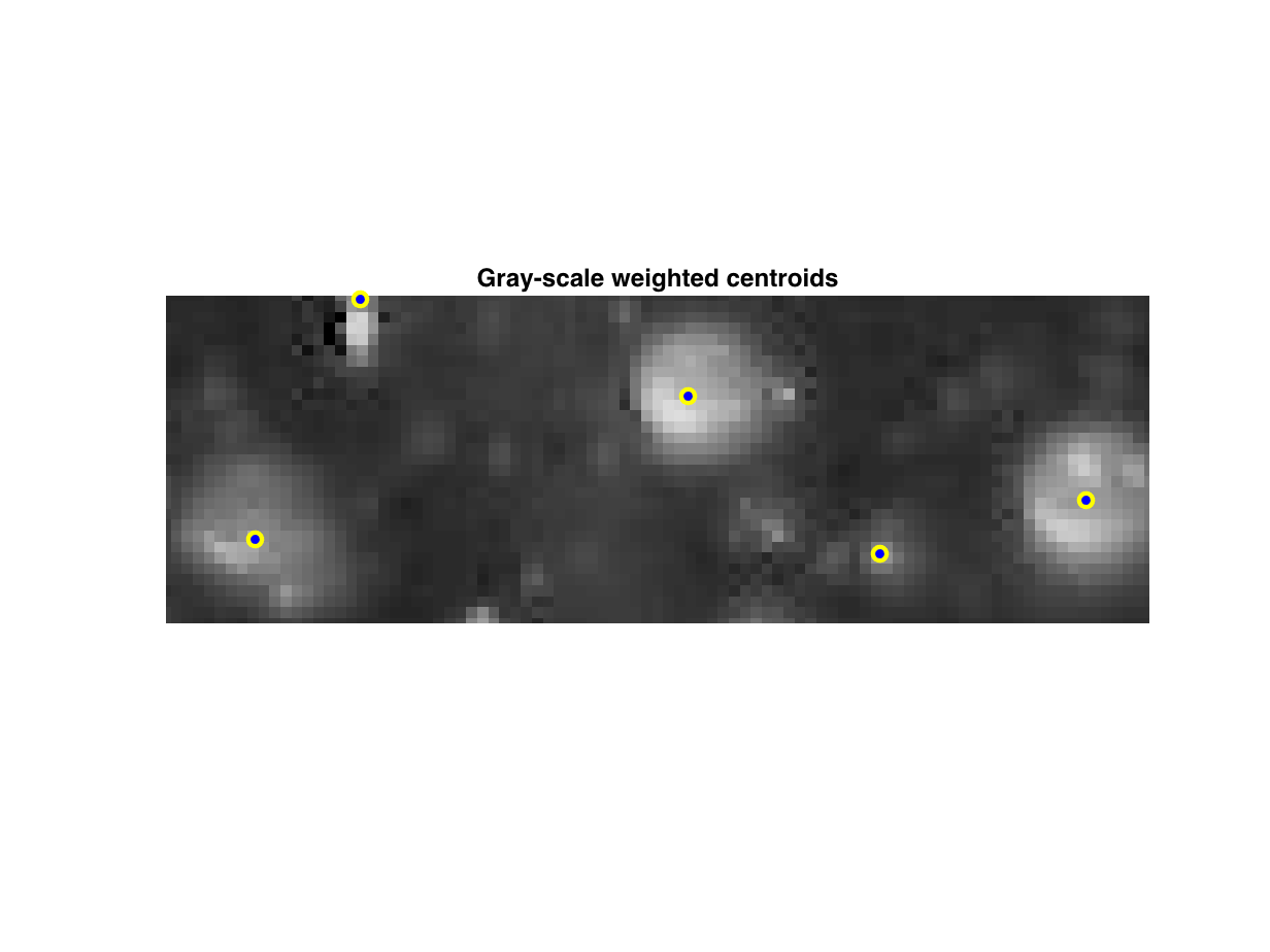
props = regionprops(“desk”,B_regmax,A,“WeightedCentroid”)
And this is one approach to visualize the outcomes:
plot(props.WeightedCentroid(:,1),props.WeightedCentroid(:,2),…
LineStyle=“none”, Marker=“o”, MarkerEdgeColor=“y”,…
maintain off
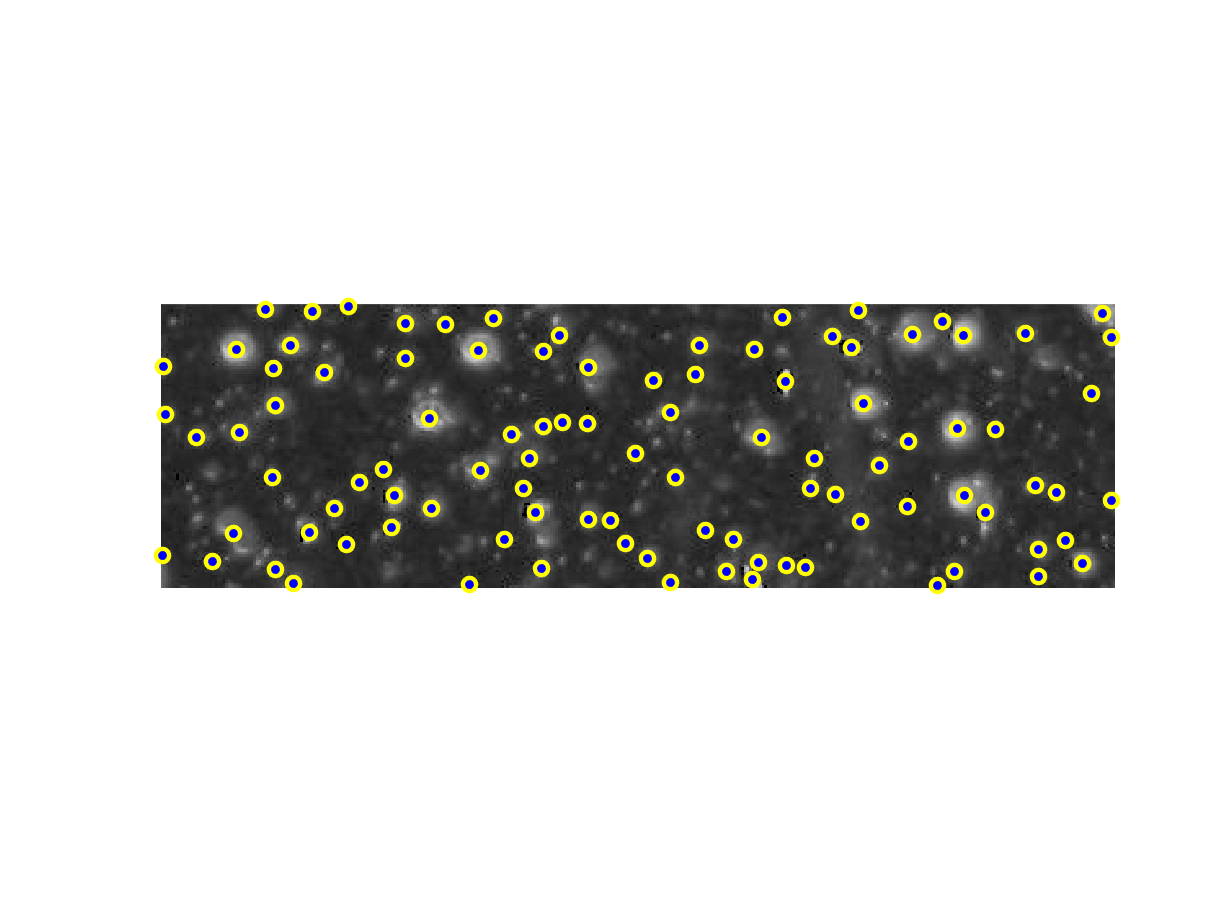
title(“Grey-scale weighted centroids”)