


The 4-by-4 matrices within the panels on the next screenshots are on the coronary heart of pc graphics. They describe objects shifting in three-dimensional house and are important to MATLAB’s Deal with Graphics, to CAD (Pc Added Design) packages, to CGI (Pc Graphics Imagery) in movies, and to hottest video video games.
Contents
Grafix 2.0
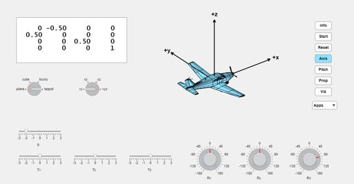
Right here is the opening display screen from model 2.0 of Grafix, my software for investigating the matrices concerned in 3-D pc graphics. The MATLAB code for Grafix is availble right here.
I’m within the matrix within the panel, which I name M. Many matrices like this one describe the dyamic transformations to be made on a set of goal objects in a posh three-dimensional scene. This specific M is the product of a scaling and a rotation that leads to the dimensions and orientation of the aircraft proven.
I additionally need to level out the coordinate axes getting used. That is view(3), MATLAB’s default 3-D cordinate system. The optimistic $x$-axis goes up and to the fitting on the display screen, the optimistic $y$-axis up and to the left, and the optimistic $z$-axis goes straight up.
Rotations
The homogeneous coordinates system utilized in trendy pc graphics makes it attainable to explain rotations, translations and plenty of different operations with 4-by-4 matrices. These matrices function on vectors with the place of an object within the first three parts and, for now, a one because the fourth element, eg. [ $x$, $y$, $z$, 1 ]’,
Rotations are described by merchandise of those matrices, every of which operates on solely two of the primary three parts of the vector. The primary matrix, $R_x$, leaves $x$ unchanged whereas it rotates $y$ and $z$. The second matrix, $R_y$, leaves $y$ unchanged whereas it rotates $x$ and $z$. And the third matrix, $R_z$, leaves $z$ unchanged whereas it rotates $x$ and $y$.
$$ R_x(theta) = left[ begin{array}{rrrr}
1 & 0 & 0 & 0
0 & cos{theta} & -sin{theta} & 0
0 & sin{theta} & cos{theta} & 0
0 & 0 & 0 & 1
end{array} right] $$
$$ R_y(theta) = left[ begin{array}{rrrr}
cos{theta} & 0 & -sin{theta} & 0
0 & 1 & 0 & 0
sin{theta} & 0 & cos{theta} & 0
0 & 0 & 0 & 1
end{array} right] $$
$$ R_z(theta) = left[ begin{array}{rrrr}
cos{theta} & -sin{theta} & 0 & 0
sin{theta} & cos{theta} & 0 & 0
0 & 0 & 1 & 0
0 & 0 & 0 & 1
end{array} right] $$
Pitch, Roll, and Yaw
The phrases pitch, roll and yaw are sometimes used to explain the movement of automobiles like plane, marine craft, and spacecraft. Pitch is $R_x$, rotation in regards to the $x$-axis.

Roll is $R_y$, rotation in regards to the $y$-axis.

And yaw is $R_z$, rotation in regards to the $z$-axis.

Translations
Translations are described by matrices with values within the fourth column. Multiplying a vector by one among these matrices produces a translation within the path of the corresponding axis.
$$ T_x(delta) = left[ begin{array}{rrrr}
1 & 0 & 0 & delta
0 & 1 & 0 & 0
0 & 0 & 1 & 0
0 & 0 & 0 & 1
end{array} right] $$
$$ T_y(delta) = left[ begin{array}{rrrr}
1 & 0 & 0 & 0
0 & 1 & 0 & delta
0 & 0 & 1 & 0
0 & 0 & 0 & 1
end{array} right] $$
$$ T_z(delta) = left[ begin{array}{rrrr}
1 & 0 & 0 & 0
0 & 1 & 0 & 0
0 & 0 & 1 & delta
0 & 0 & 0 & 1
end{array} right] $$
Whereas it’s true that translations might be completed just by including the increment to the desired coordiate, using matrix multiplication permits translations to be mixed in a uniform manner with rotations and different operations. The arithmetic models on immediately’s Graphics Processing Models, GPUs, are designed to do 4-by-4 matrix multiplications at speeds a whole bunch of occasions sooner than basic objective Central Processing Models, CPUs.
Horizontal and Vertical
Impressed by David Singmaster’s notation for Rubik’s cubes, L, R, B, F, U, and D, we are able to use the descriptive phrases left and proper for horizontal movement within the $x$ path; again and forth for horizontal movement within the $y$ path; and up and down for vertical movement within the $z$ path.
$T_x$, left and proper.
$T_y$, backwards and forwards.
$T_z$, up and down.
Scalings
This matrix applies a single scaling issue to all three axes.
$$ S(sigma) = left[ begin{array}{rrrr}
sigma & 0 & 0 & 0
0 & sigma & 0 & 0
0 & 0 & sigma & 0
0 & 0 & 0 & 1
end{array} right] $$
Bigger and Smaller
$S$
Options
Refresh your browser to syncronize the animations.
Obtain your individual self-archiving copies of
Revealed with MATLAB® R2023a