MATLAB with TensorFlow from Your Jupyter Pocket book » Synthetic Intelligence

The MATLAB Kernel for Jupyter® (GitHub: jupyter-matlab-proxy) was launched just a few months in the past. The MATLAB Kernel for Jupyter now helps Home windows®, along with MacOs and Linux®. On this weblog publish, Yann Debray and I’ll present how one can create a deep studying mannequin and convert it from MATLAB to TensorFlow™ by operating MATLAB code and practice the transformed TensorFlow mannequin by operating Python code; all from the similar Jupyter pocket book.

Most significantly, on this weblog publish we are going to present how straightforward it’s to change between MATLAB and Python code in your Jupyter pocket book. As a result of we don’t have to change coding setting – we simply swap kernels – this was the quickest mannequin alternate prototype that we have now created to date.

For demonstration functions, we made the instance on this publish light-weight and straightforward to observe. However you possibly can prolong this instance to extra sophisticated workflows, similar to:

Set Up

Earlier weblog posts on the MATLAB Kernel for Jupyter confirmed learn how to use the kernel in Home windows and Linux. On this weblog publish, we used a MacBook to execute the workflow. The preliminary setup occurs on the MacOs terminal. First, set up the MATLAB Kernel for Jupyter.

pip set up jupyter-matlab-proxy

The MATLAB executable isn’t essentially on the system path (not less than it was not on my Mac), so we run the next command.

sudo ln -s /Purposes/MATLAB_R2023a.app/bin/matlab  /usr/native/bin

Verify that each one the instruments are put in as anticipated. After you confirm that the fitting model of Python and all the required libraries are put in (and the MATLAB executable is on the trail), open Jupyter pocket book. There are different methods to begin up a Jupyter pocket book, for instance by utilizing CPython.

Now, we’re able to run MATLAB and Python code from the identical Jupyter pocket book.

Create Mannequin with MATLAB Kernel

First, we’re going to create an LSTM mannequin in MATLAB. In your Jupyter pocket book, specify your kernel as MATLAB. This can be a one-click course of.

You possibly can run the next MATLAB code the identical method you’d from every other MATLAB setting, for instance from MATLAB desktop and MATLAB On-line.

Create Layer Graph

Create a protracted short-term reminiscence (LSTM) community to categorise sequence knowledge. An LSTM community takes sequence knowledge as enter and makes predictions based mostly on the person time steps of the sequence knowledge.

inputSize = 12;
numHiddenUnits = 100;
numClasses = 9;

layers = [
       sequenceInputLayer(inputSize)
       bilstmLayer(numHiddenUnits,OutputMode="last")
       fullyConnectedLayer(numClasses)
       softmaxLayer];

lgraph = layerGraph(layers);

Create Knowledge Set

Load the Japanese Vowels coaching knowledge set. XTrain is a cell array containing 270 sequences of dimension 12 and ranging size. YTrain is a categorical vector of labels “1”,”2″,…”9″, which correspond to the 9 audio system. To be taught extra in regards to the knowledge set, see Sequence Classification Utilizing Deep Studying.

[XTrain,YTrain] = japaneseVowelsTrainData;

Put together the sequence knowledge in XTrain for padding.

numObservations = numel(XTrain);
for i=1:numObservations
    sequence = XTrain{i};
    sequenceLengths(i) = measurement(sequence,2);
finish

[sequenceLengths,idx] = kind(sequenceLengths);
XTrain = XTrain(idx);
YTrain = YTrain(idx);

Pad XTrain alongside the second dimension.

XTrain = padsequences(XTrain,2);

Permute the sequence knowledge from the Deep Studying Toolbox™ ordering (CSN) to the TensorFlow ordering (NSC), the place C is the variety of options of the sequence, S is the sequence size, and N is the variety of sequence observations. For extra info on dimension ordering for various deep studying platforms and knowledge varieties, see Enter Dimension Ordering.

XTrain = permute(XTrain,[3,2,1]);
YTrain = double(YTrain)-1;

Save the coaching knowledge to a MAT file, so you should use them to coach the exported TensorFlow community utilizing Python code.

filename = "training_data.mat";
save(filename,"XTrain","YTrain")

I want the variables weren’t misplaced once I swap between MATLAB and Python code within the Jupyter pocket book. However it could be similar if I used to be going to depart any MATLAB setting for a Python setting.

Convert Mannequin from MATLAB to TensorFlow

Export the layer graph to TensorFlow. The exportNetworkToTensorFlow operate saves the TensorFlow mannequin within the Python bundle myModel.

exportNetworkToTensorFlow(lgraph,"./myModel")

Prepare Mannequin with Python Kernel

Then, we’re going to practice the exported TensorFlow mannequin utilizing Python. Specify your kernel as Python 3.

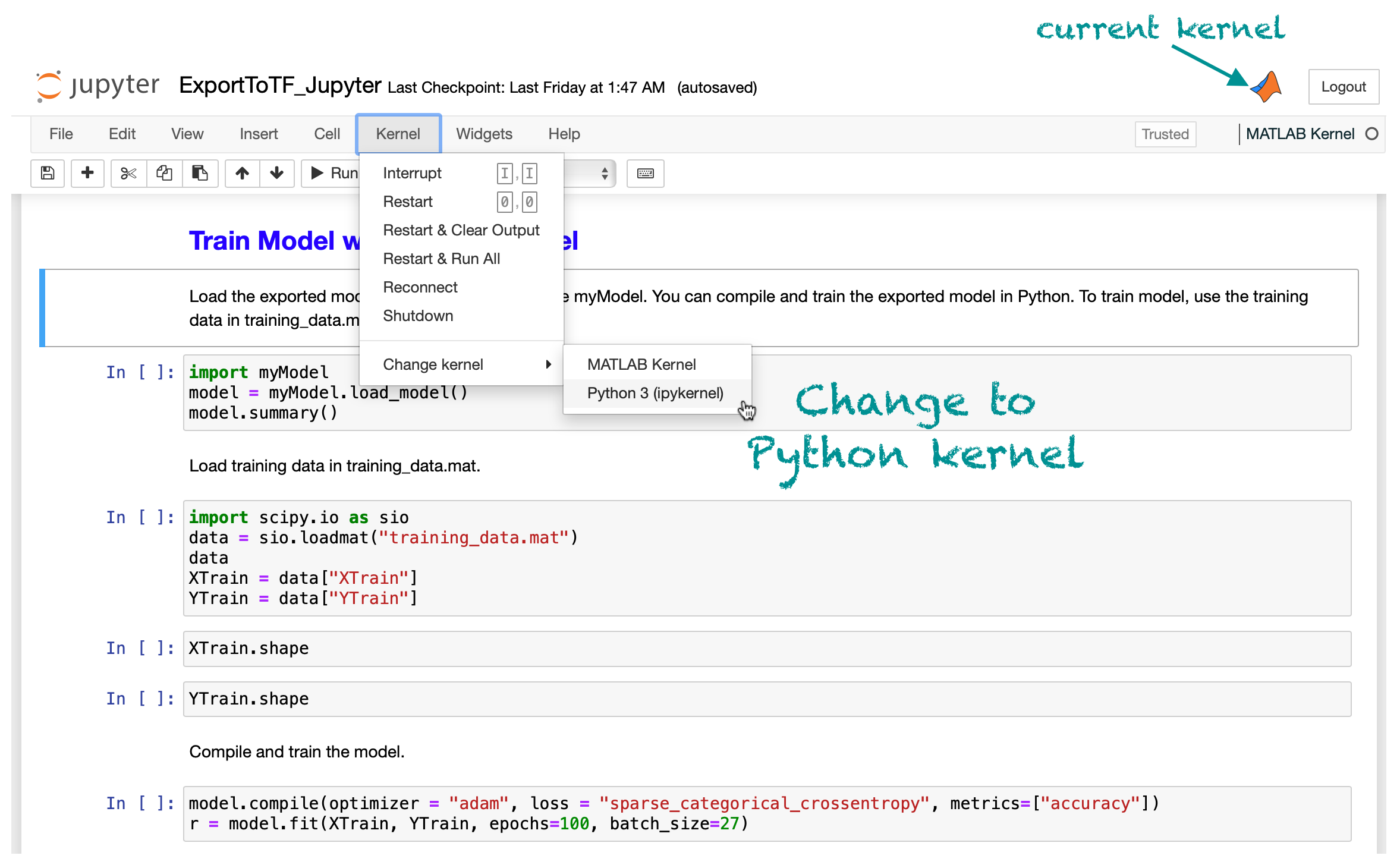Load the exported mannequin from the Python bundle myModel.

import myModel
mannequin = myModel.load_model()
mannequin.abstract()

Load the coaching knowledge in training_data.mat.

import scipy.io as sio
knowledge = sio.loadmat("training_data.mat")
XTrain = knowledge["XTrain"]
YTrain = knowledge["YTrain"]

Compile and practice the mannequin.

mannequin.compile(optimizer = "adam", loss = "sparse_categorical_crossentropy", metrics=["accuracy"])
r = mannequin.match(XTrain, YTrain, epochs=100, batch_size=27)

Save the coaching historical past to a MAT file. I solely want to do that as a result of I’m going to make use of the info in MATLAB within the subsequent part.

sio.savemat("training_history.mat",{"training_history":r.historical past})

Plot Metrics with MATLAB Kernel

Now, we’re switching again to MATLAB kernel to plot coaching metrics. We’re going to create a quite simple plot that you might create both with MATLAB or Python. For extra sophisticated deep studying workflows and visualizations (for instance, semantic segmentation), I discover that MATLAB provides extra choices and simpler to implement visualizations. Additionally, I don’t want to put in any extra Python libraries for plotting.

Nonetheless, particularly on this case, the purpose is that when it’s really easy to change between MATLAB and Python, why not simply select probably the most pure choice for you.

Load the coaching historical past.

load("training_history.mat")
historical past = struct(training_history)

Plot the loss and accuracy.

tiledlayout(2,1,TileSpacing="tight")

nexttile
plot(historical past.accuracy)
xlabel("Epochs")
ylabel("Accuracy")

nexttile
plot(historical past.loss)
xlabel("Epochs")
ylabel("Loss")

Conclusion

Collaboration, integration, and easy accessibility are key for growing AI-driven functions. On the AI weblog, we have now beforehand talked about learn how to and why use MATLAB with TensorFlow or PyTorch. The Jupyter integration makes it even simpler to make use of completely different deep studying instruments collectively, particularly for prototyping and preliminary growth. There’s nonetheless a guide component in switching between kernels (that means you possibly can’t run all of the pocket book cells), so we’d think about different choices to run MATLAB and Python code collectively for a plug-and-play model of the code.

Learn Extra on MATLAB and Python Integration

Take a look at earlier weblog posts on learn how to use MATLAB with TensorFlow and PyTorch, and the discharge of MATLAB kernel for Jupyter: