For immediately’s weblog submit,
Veer Alakshendra is glad to host
Tom Teasdale from the
UPBracing Formulation Scholar group. Tom is right here to debate concerning the instrument that he has developed for tire modeling.
Introduction
This weblog submit will briefly introduce Magic Formulation Tire and a brand new,
open-source MATLAB instrument for creating, becoming, and evaluating Magic Formulation Tire fashions. It’s tailor-made for college kids making an attempt to implement tire fashions utilizing information from the FSAE Tire Take a look at Consortium (
FSAE TTC). You’ll be able to export your fitted mannequin as a TIR-file or as a struct to make use of exterior of this instrument.
Motivation
Are you a scholar collaborating within the Formulation Scholar (FSAE) competitors? In case your reply is sure, you know the way closely your automobile is influenced by your tires. Limiting the utmost transmissible power of your engine (or motors) to the highway, tire traits ought to be understood and in comparison with make a certified tire alternative. You may also be growing a Car Dynamics Management algorithm or a high-fidelity car mannequin in MATLAB/Simulink for which you additionally want a mannequin illustration of your automobile’s tire. As an lively scholar in Formulation Scholar myself, these had been the standard challenges we needed to face at my group
UPBracing.
Fortunately, Formulation Scholar groups can achieve entry to high-quality tire information by changing into members of the
FSAE Tire Take a look at Consortium. For a small membership payment, you possibly can obtain full information of most Formulation Scholar tires which we will then use to create extremely correct and computationally environment friendly, empirical tire fashions.
Magic Formulation Tire shouldn’t be the one empirical tire modeling strategy on the market. It’s only certainly one of many. Nonetheless, additionally it is the preferred one (neglecting the linear tire mannequin), and for good causes. It may be understood as a sophisticated model of the well-known, traditional Magic Formulation.
$ y = D cdot sin bigg( C cdot arctan Huge( B cdot x – Ebig( B cdot x – arctan(B cdot x) massive) Huge) bigg) $
the place y is the output variable (e.g. lateral tyre power) and x the enter variable (e.g. slip angle). B, C,D and E are the tuning parameters.
For an instance of how one can match the traditional Magic Formulation to information, you possibly can consult with
Analyzing Tire Take a look at Knowledge, a weblog submit by MathWorks workers. Of their case, the becoming leads to a big interpolation grid which alters the parameters relying on the present steady-state situations. However interpolation grids will be disadvantageous, particularly the place execution velocity issues and they’re additionally exhausting to change after the becoming course of.
A extra superior model of the classical Magic Formulation is the semi-empirical Magic Formulation mannequin with round 100 parameters. Semi-empirical implies that the mannequin incorporates data about tire dynamics in its equations and isn’t purely empirical as, for instance, a polynomial mannequin. Subsequently, semi-empirical Magic Formulation fashions may realistically extrapolate tire traits utilizing the so-called
similarity methodology. That is very helpful, as we often don’t have test-bench information for each doable steady-state. The
TTC for instance solely exams slip angles as much as about 6 levels. Though the mannequin appears actually advanced with over 100 parameters to tune, we often solely want a fraction of these for an amazing model-data-fit. However, to be honest, it may be a bit cumbersome to construct Magic Formulation Tire fashions with simply MATLAB scripts, particularly if you wish to manually tune parameters. I hope that my instrument may help college students in that regard.
Within the following, any reference to Magic Formulation or Magic Formulation Tire implies its semi-empirical type.
Methodology
The Magic Formulation Tire Device showcased right here will be understood as an open-source various to a number of business resolution to becoming Magic Formulation Tire fashions to information. It acts as a graphical
wrapper to the intently associated mission Magic Formulation Tire
MATLAB Library, which is a group of command-line instruments. This implies, that just about all the pieces accomplished by the GUI will be accomplished with simply the library within the MATLAB console. It additionally implies that the Magic Formulation Tire equations used within the GUI for becoming are the identical as within the library. So the fitted parameter set yields the identical leads to the GUI as with the Command-Line instruments within the Magic Formulation Tire
MATLAB Library.
By the best way, the analysis capabilities within the library talked about above are code-generation appropriate and have been used for that function at
UPBracing. So be at liberty to suit your mannequin utilizing the GUI and consider it utilizing the library in your code-generation tasks.
Implementing Magic Formulation Tire
For individuals who wish to perceive the implementation of Magic Formulation Tire mannequin, I’ll present a brief abstract. Right here the definitive reference is the ebook
Tire and Car Dynamics by Hans B. Pacejka (2012). In chapter 4.3.2. you will see the complete set of equations. You must also hold the MF-Tyre/MF-Swift handbook close by as a kind of cheatsheet for the
parameters. Implementing these is fairly simple. Let’s take a peak on the
source-code for
Fx0, which calculates longitudinal tire power for pure longitudinal slip.
operate [Fx0,mux,Cx,Dx,Ex] = Fx0(p,longslip,inclangl,stress,Fz)
FNOMIN = p.FNOMIN.*p.LFZO;
dfz = (Fz-FNOMIN)./FNOMIN;
dpi = (pressure-p.NOMPRES)./p.NOMPRES;
Fx0 = Dx.*sin(Cx.*atan(Bx.*longslip-Ex.*(Bx.*longslip-atan(Bx.*longslip))))+SVx;
The parameter names have been carried out in accordance with the Magic Formulation Tire/MF-Swift handbook and variable names attempt to observe Pacejka’s ebook intently. Apart from that, you solely should translate the maths from the ebook into MATLAB code.
Creating the Fitter
In
Analyzing Tire Knowledge the
lsqcurvefit operate is used to suit the Magic Formulation Tire mannequin to information. Because the identify suggests, it minimizes the squared sum of errors. The Magic Formulation Tire Device makes use of the Fitter included within the Magic Formulation Tire
MATLAB Library. It additionally makes use of a least-squares strategy however makes use of the
fmincon operate as a substitute. It’s because I additionally wished to implement nonlinear constraints, as sure variables of Magic Formulation Tire ought to at all times be inside sure bounds. For instance, Pacejka’s ebook says that
$ $$ C_x = p_{Cx1} cdot lambda_{Cx} > 0 D_x = mu_{x} cdot F_z cdot zeta_1> 0 E_x = … leq 1 $$ $
C_x and D_x have to be higher than zero. This may be carried out as a nonlinear constraint within the fitter (see supply code).
[~,~,Cx,Dx,Ex] = mftyre.v62.equations.Fx0(params,longslip,inclangl,stress,Fz);
c = [-Cx+eps;-Dx+eps;Ex-1];
Right here
c is an output of the operate deal with handed to
fmincon as a nonlinear constraint (see
nonlcon). Subsequent, we have now to think about the order by which the mannequin is fitted to the info. Assuming that we have now separated our time sequence information into steady-state situations, which means that we have now remoted information arrays the place every enter will be thought-about fixed (aside from one sweeping variable like slip ratio or slip angle), we will do the next.
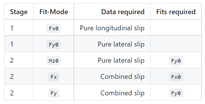
This checklist is incomplete, as Magic Formulation Tire can mannequin extra outputs, however that is ample for demonstration. This desk exhibits that we should always at all times match the mannequin to pure slip situations first (Fx0, Fy0) after which transfer on to the opposite equations. The order naturally comes from the dependencies of the equations. Fx makes use of Fx0 and solely applies a scaling time period to it, similar for Fy. Notice that it doesn’t matter whether or not you match Fx0 or Fy0 first, similar for Fx and Fy. The order described right here can also be carried out within the fitter, which means that if you choose a number of fit-modes within the GUI, the fitter will proceed in phases.
Constructing the GUI
My strategy to constructing the GUI was utilizing the
customized UI part class offered by MATLAB to develop a modularized utility with out
AppDesigner. Constructing the app through the use of customized elements makes it very simple to focus solely on part of the app. You’ll be able to execute particular person UI elements in isolation and see if any bugs come up. It isn’t essential to at all times run the complete app when growing customized UI part lessons.
I nonetheless use AppDesigner to create Mockups shortly and see if my deliberate UI appears to be like good, however I want to not use it for the ultimate utility, as AppDesigner limits my freedom to decide on property entry ranges, stopping me from creating elements in loops and extra. Nonetheless, it ought to be famous that beginning with R2021a,
now you can use customized UI elements in AppDesigner. This may resolve a number of the points I’ve had prior to now, however I haven’t tried this but.
App Demonstration
I’ll now give an illustration of the core workflow with information from the FSAE Tire Take a look at Consortium. The info has been obscured and de-identified to adapt with the license settlement.
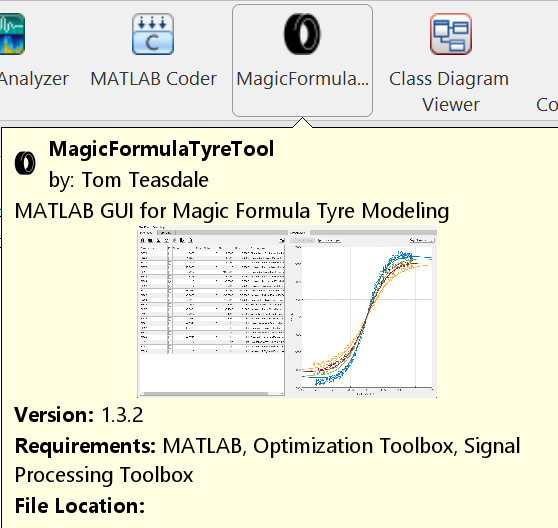
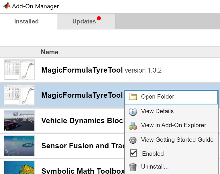
Set up the App
There are a number of methods to put in the app, however the steered manner is to obtain it from
FileExchange. Alternatively, you possibly can obtain the newest launch from
GitHub, however new releases are synced to FileExchange anyway. Obtain and set up the toolbox (
*.mltbx) which additionally contains the app. You’ll be able to then begin the instrument out of your app catalog.
Import Tire Knowledge
First, we have to purchase measurement information. In case you are a member of the
FSAE TTC, you possibly can proceed to their discussion board and obtain information from there. Please solely use information formatted as MAT and in SI models, in any other case, the pre-installed parsers will fail.
Usually, TTC information is cut up into two sorts of exams
Drive/Brake is a maneuver with both zero slip angle or fixed slip angles (steering angles). Whereas all different inputs are held fixed, the slip ratio is swept (by driving and braking the tire). Cornering doesn’t contemplate slip ratio in any respect and solely sweeps slip angle whereas all different inputs are fixed. As you possibly can see, to suit an entire Magic Formulation Tire mannequin, you want each the Drive/Brake and Cornering dataset for a given tire. You’ll be able to observe this instance through the use of the de-identified and obscured information included within the put in toolbox. Merely navigate to the toolbox folder, the place you will see instance information below doc/examples/fsae-ttc-data/, in case you don’t have entry to the TTC (but). Simply take into account that the tire traits have been modified and the ensuing mannequin will behave like an actual tire.
Now navigate to the Tyre Knowledge tab and observe the import course of as proven.
Configure and Run Fitter
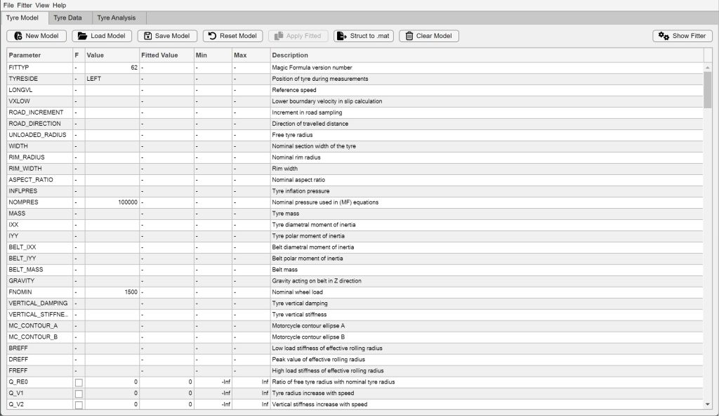
First, we have to create a brand new tire mannequin. For this, merely navigate again to the Tyre Mannequin tab and click on New Mannequin, select a file to save lots of to after which you must see the next default mannequin.
We are able to navigate to the Tyre Evaluation tab and see how nicely this mannequin matches the info. Spoiler alert: it doesn’t which is sensible, as we haven’t fitted it but.
Subsequent, we have now to configure the fit-modes. A fit-mode on this context is the equation we’re going to match. As defined earlier, totally different equations require totally different information to be fitted. For instance, becoming Fx0 requires information with no slip angle (pure longitudinal slip). In any case, you must at all times match the modes Fx0 and Fy0 first. So let’s do this. Navigating again to the Tyre Mannequin tab, we will modify the fit-modes and begin becoming.
After I seen that the target operate was reducing very slowly, I canceled the method. You don’t lose the present state of fmincon although, and the final iteration is saved. Notice that I additionally canceled earlier than Fy0 was fitted, so solely Fx0 ought to have been improved. We are able to now take a look at the fitted values and append them to our mannequin.
In case you don’t belief the fitted values, you may additionally manually switch them by typing into the worth discipline.
Confirm Mannequin-Knowledge-Match
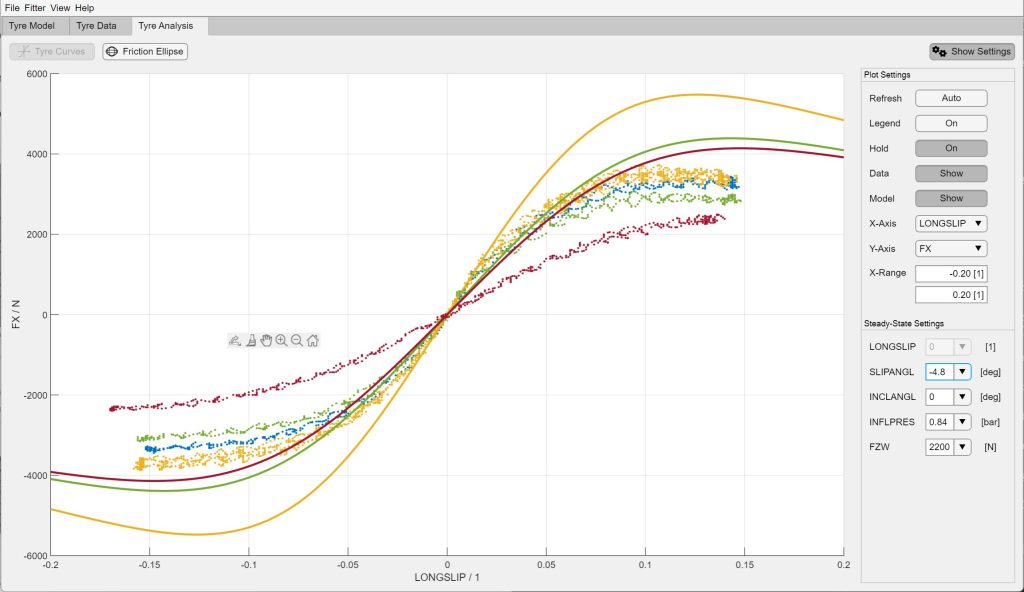
Allow us to navigate once more to the Tyre Evaluation tab and plot just a few steady-state situations to confirm the mannequin match.
The match shouldn’t be excellent, however passable. Discover that we have now not fitted Fy0, Fx and Fy but, so we should always anticipate unhealthy outcomes for these modes.
Tuning the Mannequin Manually
In case you wish to mess around with the mannequin and shortly see the outcomes, I recommend altering the window format and utilizing the Auto-Refresh possibility of the plot. It is a nice approach to perceive the which means and results of the mannequin parameters. It is usually a vital step in case your purpose is an ideal match. The fitter is nice, however not excellent.
Export Fitted Tire Mannequin
Now you can both export the mannequin as a TIR-file which is each nice for saving and re-importing the mannequin to the Magic Formulation Tire instrument, but additionally the interface to many business instruments available in the market (ADAMS, Siemens NX, Simulink, and many others). The exported file will look one thing like this
[LONGITUDINAL_COEFFICIENTS]
Alternatively, you possibly can select to export as MAT, which can then convert the tire mannequin parameters to a struct and reserve it to the MAT file. This export is sensible if it is advisable use the Magic Formulation Tire mannequin inside MATLAB, utilizing the
mftyre.v62.eval operate from the
library for instance.
Notice that at present it isn’t doable to import the MAT file into the instrument, so at all times hold the TIR-file saved other than the MAT export.
Outcomes and conclusion
We now have now fitted our Magic Formulation Tire mannequin to actual information from the FSAE TTC. The entire course of took lower than 5 minutes, though we have now skipped some steps for demonstration functions. As talked about earlier than, you possibly can both use the TIR-file for third-party simulations or use the exported struct in MATLAB immediately. If you wish to use the Magic Formulation Tire
MATLAB library, use the next syntax.
[Fx,Fy] = mftyre.v62.eval(p,slipangl,longslip,inclangl,inflpres,FZW,tyreSide)
The place p is the exported parameter struct. In my expertise, this analysis operate has confirmed to be very quick in execution with little overhead. Because it was created to be used in real-time management and estimation algorithms in thoughts, this was a vital situation.
Nonetheless, the equations are at present not full. They don’t calculate the moments
Mz0,
Mz,
Mx and
My for instance. Additionally, the flip slip has been uncared for. As an amazing various, you may as well use the favored
mfeval mission created by
Marco Furlan to guage the exported TIR-file. Simply take into account that the GUI additionally doesn’t match the modes talked about.
output = mfeval(TIRfile, inputs, useMode);
I hope that this instrument can profit some college students in Formulation Scholar to lastly create an in depth tire mannequin themselves!
Future scope
The Magic Formulation Tire Device appears to be working nice already I’ve been advised by just a few beta-testers. However there are nonetheless some options deliberate for the close to future.
- Compatibility with older variations of Magic Formulation Tire
- Extra Evaluation choices (e.g. Kamm-Circle)
- High quality-of-Life enhancements (usability)
- Weighting capabilities for Fitter (placing extra weight on decrease masses for instance)
If you wish to be saved within the loop, contemplate
starring my
GitHub repository or score my instrument on
FileExchange. Each will hold me motivated so as to add options to the instrument. In case you wish to contribute your self, please be at liberty to take action. Get in contact with me and we’ll discover a approach to collaborate!
Acknowledgments
I additionally wish to acknowledge
Marco Furlan with whom I had an pleasurable trade on LinkedIn. He developed the talked about
mfeval toolbox, which remains to be the definitive open-source MATLAB implementation of Magic Formulation Tire in the marketplace. His mission helped me get began with Magic Formulation Tire nearly three years again and was enormously appreciated.
Lastly, I wish to acknowledge the beforehand reference weblog submit by MathWorks workers known as
Analyzing Tire Take a look at Knowledge from which I realized the genius manner of utilizing the MATLAB operate
histcounts to routinely separate time sequence information into steady-states. Their approach has been used to develop the measurement import parsers.


