

⚔️ Programming Problem: Given an integer n that may very well be very excessive (e.g., n=1000000). The best way to initialize a Python dictionary of dimension n that’s quick, straightforward, and environment friendly?
Subsequent, you’ll be taught the 5 primary methods to unravel this and examine their efficiency on the finish of this text. Apparently, the winner Methodology 4 is 38% quicker than the slowest Methodology 5 and 14% quicker than the following quickest.
Scroll right down to see the profitable technique that’s each straightforward and maximally environment friendly! 🚀
Methodology 1: Primary For Loop
A easy and simple—however not tremendous concise—strategy to create and initialize a dictionary of dimension n is to make use of a easy for loop to replenish an initially empty dictionary by utilizing dictionary assignments comparable to d[i] = None within the loop physique.
Right here’s a easy code snippet utilizing this strategy:
def init_dict_1(n):
    ''' Initialize a dictionary with n key-value pairs. '''
    d = {}
    for i in vary(n):
        d[i] = None
    return d
The output:
print(init_dict_1(100))

{0: None, 1: None, 2: None, 3: None, 4: None, 5: None, 6: None, 7: None, 8: None, 9: None, 10: None, 11: None, 12: None, 13: None, 14: None, 15: None, 16: None, 17: None, 18: None, 19: None, 20: None, 21: None, 22: None, 23: None, 24: None, 25: None, 26: None, 27: None, 28: None, 29: None, 30: None, 31: None, 32: None, 33: None, 34: None, 35: None, 36: None, 37: None, 38: None, 39: None, 40: None, 41: None, 42: None, 43: None, 44: None, 45: None, 46: None, 47: None, 48: None, 49: None, 50: None, 51: None, 52: None, 53: None, 54: None, 55: None, 56: None, 57: None, 58: None, 59: None, 60: None, 61: None, 62: None, 63: None, 64: None, 65: None, 66: None, 67: None, 68: None, 69: None, 70: None, 71: None, 72: None, 73: None, 74: None, 75: None, 76: None, 77: None, 78: None, 79: None, 80: None, 81: None, 82: None, 83: None, 84: None, 85: None, 86: None, 87: None, 88: None, 89: None, 90: None, 91: None, 92: None, 93: None, 94: None, 95: None, 96: None, 97: None, 98: None, 99: None}
👉 Really helpful Tutorial: Including Components to a Python Dictionary
Methodology 2: Dictionary Comprehension
Dictionary Comprehension is a concise and memory-efficient strategy to create and initialize dictionaries in one line of Python code. It consists of two elements: expression and context.
- The expression defines find out how to map keys to values.
- The context loops over an iterable utilizing a single-line
forloop and defines whichkey:worthpairs to incorporate within the new dictionary.
Right here’s how you should use dictionary comprehension to create and initialize a dictionary of dimension n:
def init_dict_2(n):
    ''' Initialize a dictionary with n key-value pairs. '''
    return {i:None for i in vary(n)}
The output:
print(init_dict_2(100))

{0: None, 1: None, 2: None, 3: None, 4: None, 5: None, 6: None, 7: None, 8: None, 9: None, 10: None, 11: None, 12: None, 13: None, 14: None, 15: None, 16: None, 17: None, 18: None, 19: None, 20: None, 21: None, 22: None, 23: None, 24: None, 25: None, 26: None, 27: None, 28: None, 29: None, 30: None, 31: None, 32: None, 33: None, 34: None, 35: None, 36: None, 37: None, 38: None, 39: None, 40: None, 41: None, 42: None, 43: None, 44: None, 45: None, 46: None, 47: None, 48: None, 49: None, 50: None, 51: None, 52: None, 53: None, 54: None, 55: None, 56: None, 57: None, 58: None, 59: None, 60: None, 61: None, 62: None, 63: None, 64: None, 65: None, 66: None, 67: None, 68: None, 69: None, 70: None, 71: None, 72: None, 73: None, 74: None, 75: None, 76: None, 77: None, 78: None, 79: None, 80: None, 81: None, 82: None, 83: None, 84: None, 85: None, 86: None, 87: None, 88: None, 89: None, 90: None, 91: None, 92: None, 93: None, 94: None, 95: None, 96: None, 97: None, 98: None, 99: None}
👉 Really helpful Tutorial: Python Dictionary Comprehension: A Highly effective One-Liner Tutorial
Methodology 3: zip() and vary()
The zip() operate takes an arbitrary variety of iterables and aggregates them to a single iterable, a zipper object. It combines the i-th values of every iterable argument right into a tuple. Therefore, for those who go two iterables, every tuple will include two values.
You need to use the zip() operate to assemble a dictionary by first utilizing it to create an iterable of tuples utilizing zip(vary(n), [None] * n) the place the primary tuple values are the keys and the second tuple values are None. Then go the consequence into the dict() operate to create a dictionary out of it.
Right here’s how this one-liner resolution seems like:
def init_dict_3(n):
    ''' Initialize a dictionary with n key-value pairs. '''
    return dict(zip(vary(n), [None] * n))
The output:
print(init_dict_3(100))

{0: None, 1: None, 2: None, 3: None, 4: None, 5: None, 6: None, 7: None, 8: None, 9: None, 10: None, 11: None, 12: None, 13: None, 14: None, 15: None, 16: None, 17: None, 18: None, 19: None, 20: None, 21: None, 22: None, 23: None, 24: None, 25: None, 26: None, 27: None, 28: None, 29: None, 30: None, 31: None, 32: None, 33: None, 34: None, 35: None, 36: None, 37: None, 38: None, 39: None, 40: None, 41: None, 42: None, 43: None, 44: None, 45: None, 46: None, 47: None, 48: None, 49: None, 50: None, 51: None, 52: None, 53: None, 54: None, 55: None, 56: None, 57: None, 58: None, 59: None, 60: None, 61: None, 62: None, 63: None, 64: None, 65: None, 66: None, 67: None, 68: None, 69: None, 70: None, 71: None, 72: None, 73: None, 74: None, 75: None, 76: None, 77: None, 78: None, 79: None, 80: None, 81: None, 82: None, 83: None, 84: None, 85: None, 86: None, 87: None, 88: None, 89: None, 90: None, 91: None, 92: None, 93: None, 94: None, 95: None, 96: None, 97: None, 98: None, 99: None}
👉 Really helpful Tutorial: Understanding the zip() operate in Python
Methodology 4: dict.fromkeys()
The tactic dict.fromkeys() is a really helpful technique for creating new dictionaries from a given iterable of keys. It inputs keys and possibly an elective worth, and outputs a dictionary with the desired keys, which can be mapped both to optionally specified values or to the default None worth.
def init_dict_4(n):
    ''' Initialize a dictionary with n key-value pairs. '''
    return dict.fromkeys(vary(n))
The output:
print(init_dict_4(100))

{0: None, 1: None, 2: None, 3: None, 4: None, 5: None, 6: None, 7: None, 8: None, 9: None, 10: None, 11: None, 12: None, 13: None, 14: None, 15: None, 16: None, 17: None, 18: None, 19: None, 20: None, 21: None, 22: None, 23: None, 24: None, 25: None, 26: None, 27: None, 28: None, 29: None, 30: None, 31: None, 32: None, 33: None, 34: None, 35: None, 36: None, 37: None, 38: None, 39: None, 40: None, 41: None, 42: None, 43: None, 44: None, 45: None, 46: None, 47: None, 48: None, 49: None, 50: None, 51: None, 52: None, 53: None, 54: None, 55: None, 56: None, 57: None, 58: None, 59: None, 60: None, 61: None, 62: None, 63: None, 64: None, 65: None, 66: None, 67: None, 68: None, 69: None, 70: None, 71: None, 72: None, 73: None, 74: None, 75: None, 76: None, 77: None, 78: None, 79: None, 80: None, 81: None, 82: None, 83: None, 84: None, 85: None, 86: None, 87: None, 88: None, 89: None, 90: None, 91: None, 92: None, 93: None, 94: None, 95: None, 96: None, 97: None, 98: None, 99: None}
👉 Really helpful Tutorial: Python’s Dictionary fromkeys() Methodology
Methodology 5: Easy Whereas Loop
You too can use a easy whereas loop to create a big dictionary one mapping at a time. The distinction between a whereas and a for loop (see Methodology 1) is that you simply don’t depend on the vary() operate this fashion which can take a while. The whereas loop strategy works with easy integer addition operations.
Right here’s the answer utilizing whereas:
def init_dict_5(n):
    ''' Initialize a dictionary with n key-value pairs. '''
    d = dict()
    i = 0
    whereas i<n:
        d[i] = None
        i += 1
    return d
The output:
print(init_dict_5(100))

{0: None, 1: None, 2: None, 3: None, 4: None, 5: None, 6: None, 7: None, 8: None, 9: None, 10: None, 11: None, 12: None, 13: None, 14: None, 15: None, 16: None, 17: None, 18: None, 19: None, 20: None, 21: None, 22: None, 23: None, 24: None, 25: None, 26: None, 27: None, 28: None, 29: None, 30: None, 31: None, 32: None, 33: None, 34: None, 35: None, 36: None, 37: None, 38: None, 39: None, 40: None, 41: None, 42: None, 43: None, 44: None, 45: None, 46: None, 47: None, 48: None, 49: None, 50: None, 51: None, 52: None, 53: None, 54: None, 55: None, 56: None, 57: None, 58: None, 59: None, 60: None, 61: None, 62: None, 63: None, 64: None, 65: None, 66: None, 67: None, 68: None, 69: None, 70: None, 71: None, 72: None, 73: None, 74: None, 75: None, 76: None, 77: None, 78: None, 79: None, 80: None, 81: None, 82: None, 83: None, 84: None, 85: None, 86: None, 87: None, 88: None, 89: None, 90: None, 91: None, 92: None, 93: None, 94: None, 95: None, 96: None, 97: None, 98: None, 99: None}
👉 Really helpful Tutorial: Understanding Python Loops from the Floor Up
Efficiency Analysis
We used an Intel Core i7 with 1.8GHz TurboBost as much as 4.6 GHz with 8GB DDR4 Reminiscence and 512GB storage (not that it mattered) to check every of the 5 strategies on numerous values of n—utilizing an exponentially rising operate as proven within the code under.
This allowed us to stress-test the dictionary creation capabilities mentioned on this article on giant inputs to generate dictionaries with as much as 100 million (!) entries. 😮
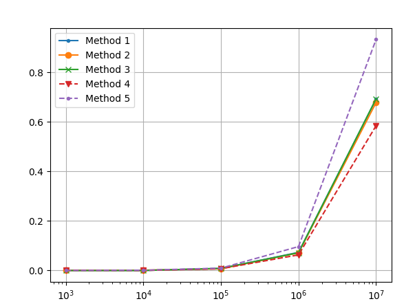
⚡ Experiment Outcomes: The output exhibits that Methodology 4 is the quickest and scaled finest, adopted by Methodology 2, Methodology 3, Methodology 1, and eventually Methodology 5 (the slowest). The winner Methodology 4 is 38% quicker than the slowest Methodology 5 and 14% quicker than the following quickest.
- Methodology 1 wanted 0.69 seconds for 100 million dict entries.
- Methodology 2 wanted 0.67 seconds for 100 million dict entries.
- Methodology 3 wanted 0.69 seconds for 100 million dict entries.
- Methodology 4 wanted 0.58 seconds for 100 million dict entries.
- Methodology 5 wanted 0.93 seconds for 100 million dict entries.
We used the next code to generate this graphic:
import time
import matplotlib.pyplot as plt


def init_dict_1(n):
    ''' Initialize a dictionary with n key-value pairs. '''
    d = {}
    for i in vary(n):
        d[i] = None
    return d


def init_dict_2(n):
    ''' Initialize a dictionary with n key-value pairs. '''
    return {i:None for i in vary(n)}


def init_dict_3(n):
    ''' Initialize a dictionary with n key-value pairs. '''
    return dict(zip(vary(n), [None] * n))


def init_dict_4(n):
    ''' Initialize a dictionary with n key-value pairs. '''
    return dict.fromkeys(vary(n))


def init_dict_5(n):
    ''' Initialize a dictionary with n key-value pairs. '''
    d = dict()
    i = 0
    whereas i<n:
        d[i] = None
        i += 1
    return d


# Efficiency Analysis
xs = []
y_1, y_2, y_3, y_4, y_5 = [], [], [], [], []
for x in [10**i for i in range(3, 8)]:
    xs.append(x)

    # Methodology 1 Elapsed Runtime:
    begin = time.time()
    init_dict_1(x)
    cease = time.time()
    y_1.append(cease - begin)

    # Methodology 2 Elapsed Runtime:
    begin = time.time()
    init_dict_2(x)
    cease = time.time()
    y_2.append(cease - begin)

    # Methodology 3 Elapsed Runtime:
    begin = time.time()
    init_dict_3(x)
    cease = time.time()
    y_3.append(cease - begin)

    # Methodology 4 Elapsed Runtime:
    begin = time.time()
    init_dict_4(x)
    cease = time.time()
    y_4.append(cease - begin)

    # Methodology 5 Elapsed Runtime:
    begin = time.time()
    init_dict_5(x)
    cease = time.time()
    y_5.append(cease - begin)


print(y_1)
print(y_2)
print(y_3)
print(y_4)
print(y_5)

plt.plot(xs, y_1, '.-', label="Methodology 1")
plt.plot(xs, y_2, 'o-', label="Methodology 2")
plt.plot(xs, y_3, 'x-', label="Methodology 3")
plt.plot(xs, y_4, 'v--', label="Methodology 4")
plt.plot(xs, y_5, '.--', label="Methodology 5")

plt.xscale('log')
plt.legend()
plt.grid()
plt.present()
In case you want the precise values in seconds, right here’s the output, one line per Methodology:
[0.0, 0.0, 0.008193492889404297, 0.07302451133728027, 0.6917409896850586]
[0.0, 0.0009975433349609375, 0.006968975067138672, 0.07086825370788574, 0.6777770519256592]
[0.0, 0.0, 0.008328437805175781, 0.07159566879272461, 0.6925091743469238]
[0.000997304916381836, 0.0, 0.006980180740356445, 0.06289315223693848, 0.5841073989868164]
[0.0, 0.0009970664978027344, 0.009291648864746094, 0.09641242027282715, 0.9321954250335693]
You may see that for the most important n=100000000, we acquire a runtime of 0.93 seconds for Methodology 5 and solely 0.58s for Methodology 4.
Abstract
The best and quickest strategy to create and initialize a dictionary with n parts is dict.fromkeys(vary(n)) that maps every integer i to the default worth None. In the event you want one other default worth (comparable to 42), simply go it as a second argument into the operate.

Whereas working as a researcher in distributed methods, Dr. Christian Mayer discovered his love for instructing pc science college students.
To assist college students attain greater ranges of Python success, he based the programming training web site Finxter.com. He’s writer of the favored programming ebook Python One-Liners (NoStarch 2020), coauthor of the Espresso Break Python collection of self-published books, pc science fanatic, freelancer, and proprietor of one of many prime 10 largest Python blogs worldwide.
His passions are writing, studying, and coding. However his best ardour is to serve aspiring coders by way of Finxter and assist them to spice up their expertise. You may be part of his free e-mail academy right here.