Extra experiments with sRGB gamut boundary in L*a*b* area » Steve on Picture Processing with MATLAB

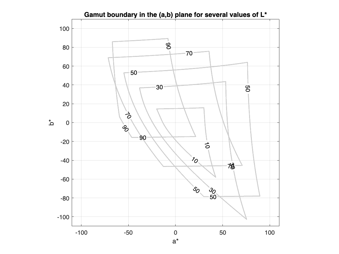
First, right here is one other strategy to talk the concept that the in-gamut space within the $ (a^*,b^*) $ airplane varies with $ L^* $ (perceptual lightness). For 9 values of $ L^* $, (10, 20, …, 90), I will compute a 2-D $ (a^*,b^*) $ gamut masks by brute-forcing it. Then, I will use overlaid contour plots to point out the variation in gamut boundaries.

[aa,bb,LL] = meshgrid(a,b,L);

rgb = lab2rgb(cat(3,LL(:,:,okay),aa(:,:,okay),bb(:,:,okay)));

masks = all((0 <= rgb) & (rgb <= 1),3) * 2 – 1 + L(okay);

contour(a,b,masks,[L(k) L(k)],LineColor=[.8 .8 .8],LineWidth=1.5,ShowText=true,…

title(“Gamut boundary within the (a,b) airplane for a number of values of L*”)

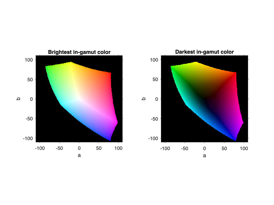
This is one other visualization idea. Individuals typically present colours on the $ (a^*,b^*) $ airplane, to provide an thought of the which means of $ a^* $ and $ b^* $, however that does not talk very nicely the concept that there are often a number of colours, corresponding to numerous $ L^* $ values, at anybody $ (a^*,b^*) $ location. Beneath, I present each the brightest in-gamut colour and the darkest in-gamut colour at every $ (a^*,b^*) $ location.

rgb = lab2rgb(cat(3,L_max,aa,bb));

imshow(rgb,XData=a([1 end]),YData=b([1 end]))

title(“Brightest in-gamut colour”)

rgb_min = lab2rgb(cat(3,L_min,aa,bb));

imshow(rgb_min,XData=a([1 end]),YData=b([1 end]))

title(“Darkest in-gamut colour”)

Subsequent, I discover myself typically wanting to attract a ray in $ L^* a^* b^* $ area and discover the gamut boundary location alongside that ray. To that finish, I wrote a easy utility operate (findNonzeroBoundary beneath) that performs a binary search to seek out the place a operate goes from optimistic to 0. Then, I wrote some nameless features to seek out the specified gamut boundary level. Particularly, I used to be on this query: For a given $ L^* $ worth and a given $ (a^*,b^*) $ airplane angle, h, what’s the in-gamut colour with the utmost chroma, c, or distance from $ (0,0) $ within the $ (a^*,b^*) $ airplane?

Honest warning: the code beneath will get tough with nameless features. You may hate it. If that’s the case, I completely perceive, and I hope you may forgive me. 🙂

I will begin by creating an nameless operate that converts from $ L^* c h $ to $ L^* a^* b^* $:

Subsequent, right here is an nameless operate that returns whether or not or not a specific $ L^* a^* b^* $ level is in gamut.

Lastly, a 3rd nameless operate makes use of findNonzeroBoundary to seek out the gamut boundary level that I am excited about.

Let’s train this operate to discover a excessive chroma darkish colour at $ h=0^{circ} $.

And here is what that colour seems to be like.

rgb_out = lab2rgb(lch2lab([L c h]));

axis off

What occurs once we attempt to discover a excessive chroma colour, on the identical hue angle, that’s shiny as a substitute of darkish?

You possibly can can see that the utmost c worth is way decrease for the upper worth of $ L^* $. What does it appear like?

rgb_out = lab2rgb(lch2lab([L c h]));

axis off

Once I was doing these experiments to arrange for this weblog put up, my authentic intent was to only present examples for a few totally different values of h and $ L^* $. However I could not cease! It was an excessive amount of enjoyable, and I stored making an attempt totally different values.

After about quarter-hour or so, I made a decision it will be greatest to jot down some easy loops to generate a comparatively giant variety of $ (L^*,h) $ combos to take a look at. This is the code to generate the excessive c colours for a wide range of $ (L^*,h) $ combos.

And here is the code to view all these colours on a grid, with labeled h and $ L^* $ axes.

rgb2 = reshape(fliplr(rgb),[],3);

p = colorSwatches(rgb2,[length(L) length(h)]);

p.XData = (p.XData – 0.5) * (dh/1.5) + h(1);

p.YData = (p.YData – 0.5) * (dL/1.5) + L(1);

title(“Highest chroma (most saturated) colours for various L* and h values”)

Utility Features