


 |
Co-author: Tom Couture
Tom Couture is the Product Supervisor for Optimization. On this weblog submit, he joins me to demonstrates methods to use the brand new MATLAB MCP Core Server to construct optimization brokers. |
If you’re like Tom, you could have most likely spent hours organising optimization issues in MATLAB—defining goal features, constraints, selecting solvers, tweaking choices. Now, what if I informed you which you can have a dialog with an AI agent that does all of this for you, like a mini Tom in your pocket, whereas truly working the optimization in your native MATLAB?
That’s the place the MATLAB MCP Core Server is available in, mixed with the highly effective Optimization Toolbox . On this submit, we’re going to stroll you thru methods to create an optimization agent that may resolve actual engineering issues—from easy constrained optimization to computationally costly CFD-based design optimization utilizing surrogate fashions.
. On this submit, we’re going to stroll you thru methods to create an optimization agent that may resolve actual engineering issues—from easy constrained optimization to computationally costly CFD-based design optimization utilizing surrogate fashions.The First Factor Your Agent Ought to Do: Test the Toolboxes
One of many first options of the MATLAB MCP Core Server I demo is the detect_matlab_toolboxes instrument. Earlier than your agent begins writing optimization code, it ought to confirm that you’ve the required toolboxes put in.
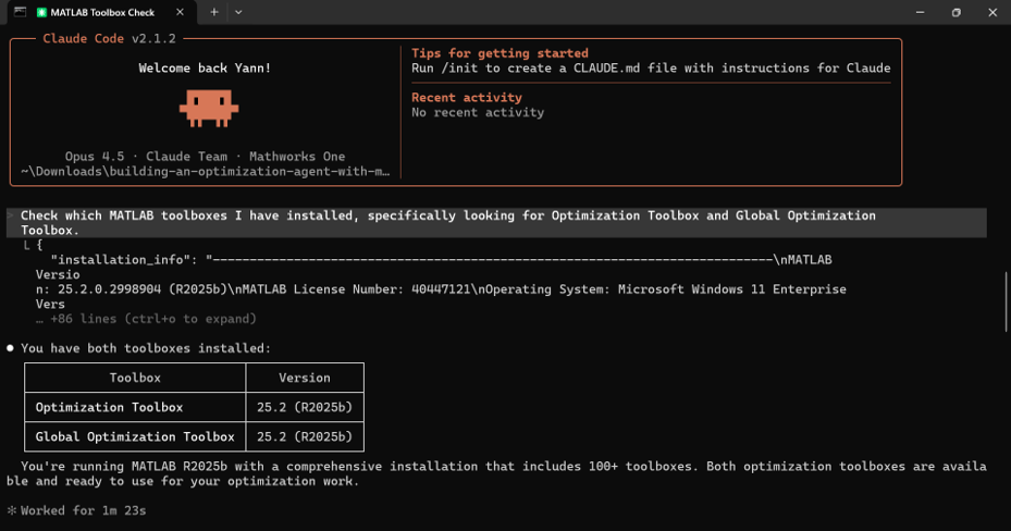
Here’s a pattern immediate to your AI assistant (Claude Desktop®, GitHub Copilot®, or any MCP-compatible shopper):
“Test which MATLAB toolboxes I’ve put in, particularly on the lookout for Optimization Toolbox and World Optimization Toolbox.”
The agent will name the detect_matlab_toolboxes instrument and return one thing like:
Optimization Toolbox – Model 25.2 (R2025b) ✓
World Optimization Toolbox – Model 25.2 (R2025b) ✓
That is essential as a result of the solver you should use relies upon completely on what you could have licensed. No Optimization Toolbox? The agent will know to fall again to fminsearch. Have World Optimization Toolbox? Nice, surrogateopt is on the desk for these costly simulations.
Instance 1: Structural Beam Design Optimization
Let me demo to you a traditional engineering optimization drawback: designing a cantilever beam for minimal weight whereas satisfying stress and deflection constraints.
The Drawback
We need to decrease the burden of an oblong cross-section beam topic to:
- Most stress constraint (should not exceed yield energy)
- Most deflection constraint (should not exceed allowable deflection)
- Bounds on width and top
Right here is the immediate I gave to Claude Code:
“I must optimize a cantilever beam design. The beam has size L=5m, carries a tip load P=10kN, made from metal with E=200 GPa and yield stress=250 MPa. I need to decrease the cross-sectional space (width × top) whereas protecting tip deflection below 10mm and max stress below the yield stress. Width needs to be between 50-200mm, top between 100-500mm. Please set this up and resolve it utilizing MATLAB.”
The agent generated and ran the next code:
% Beam optimization drawback
L = 5; % Size [m]
P = 10000; % Tip load [N]
E = 200e9; % Younger’s modulus [Pa]
sigma_yield = 250e6; % Yield stress [Pa]
delta_max = 0.010; % Max deflection [m]
% Goal: decrease cross-sectional space
goal = @(x) x(1) * x(2); % width * top
% Nonlinear constraints
nonlcon = @(x) beamConstraints(x, L, P, E, sigma_yield, delta_max);
% Bounds: [width_min, height_min] to [width_max, height_max]
lb = [0.05, 0.10]; % [m]
ub = [0.20, 0.50]; % [m]
% Preliminary guess
x0 = [0.10, 0.25];
% Clear up
choices = optimoptions(‘fmincon’, ‘Show’, ‘iter’, ‘Algorithm’, ‘sqp’);
[x_opt, fval, exitflag] = fmincon(goal, x0, [], [], [], [], lb, ub, nonlcon, choices);
fprintf(‘Optimum width: %.1f mmn’, x_opt(1)*1000);
fprintf(‘Optimum top: %.1f mmn’, x_opt(2)*1000);
fprintf(‘Optimum space: %.2f cm²n’, fval*1e4);
The constraint operate:
operate [c, ceq] = beamConstraints(x, L, P, E, sigma_yield, delta_max)
b = x(1); % width
h = x(2); % top
I = b * h^3 / 12; % Second second of space
sigma = P * L * (h/2) / I; % Max bending stress
delta = P * L^3 / (3 * E * I); % Tip deflection
c(1) = sigma – sigma_yield; % Stress constraint
c(2) = delta – delta_max; % Deflection constraint
ceq = [];
finish
The outcome? An optimum beam with width 80.2mm and top 189.4mm—satisfying each constraints on the boundary, which is strictly what you’d anticipate from a well-posed optimization drawback.
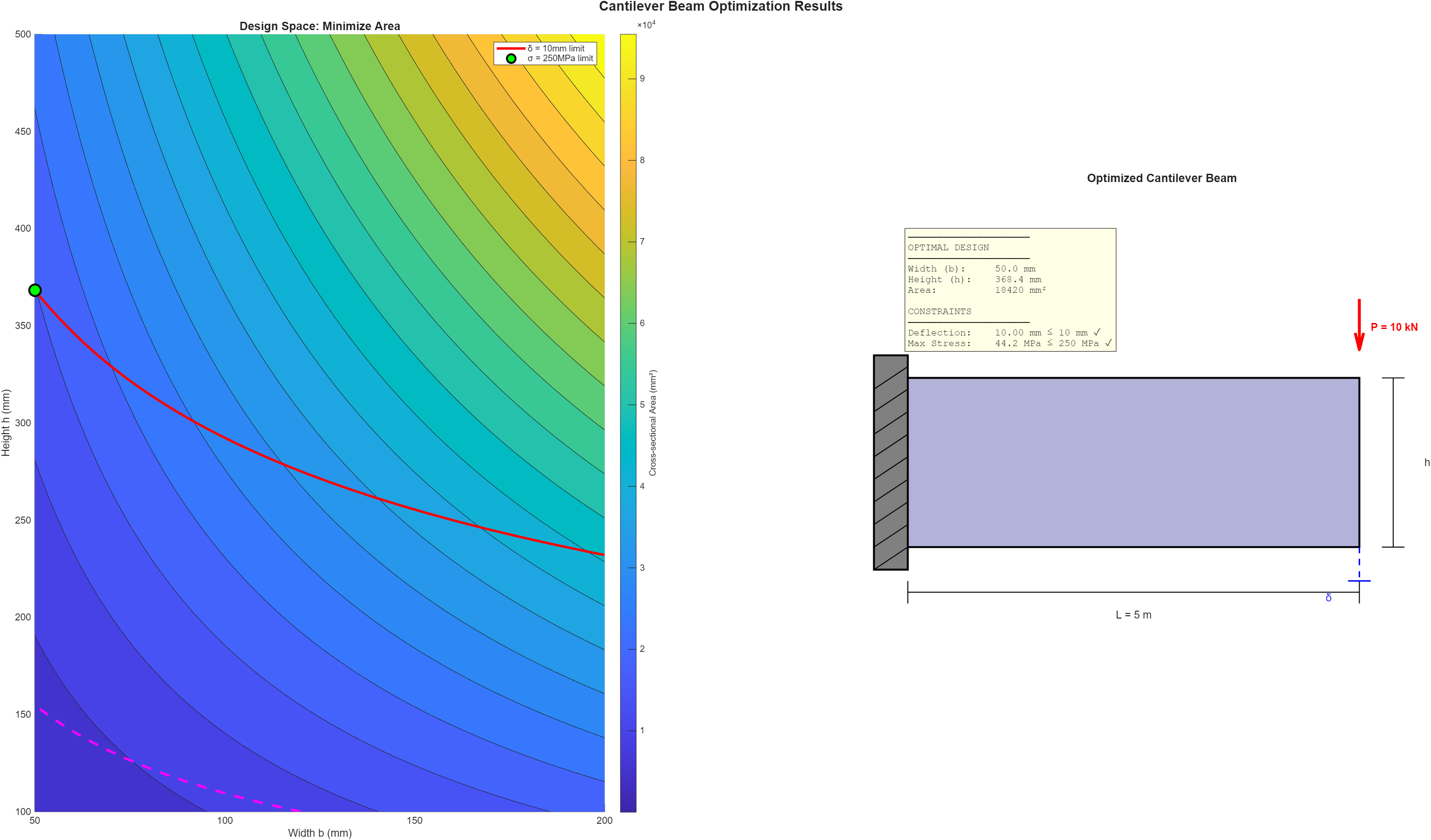
You’ll be able to check out my dialog with Claude to see a few of the rationale as to why he used a fmincon solver for this drawback:
Within the repo, I am additionally sharing a “talent” for a problem-based strategy:
Instance 2: CFD-Based mostly Optimization with Response Surfaces
Now let’s get to the enjoyable half. One among my favourite purposes of optimization in MATLAB is when you could have a computationally costly simulation—like CFD—and you want to discover optimum design parameters.
The Lid-Pushed Cavity Drawback
The lid-driven cavity is the “Whats up World” of CFD. It’s a sq. cavity the place the highest wall (the “lid”) strikes at a relentless velocity, and also you resolve the Navier-Stokes equations to seek out the circulation area. For this demo, I shall be utilizing an implementation from this drawback in pure MATLAB from my colleague Michio in Japan. The code may be discovered on GitHub: 2D Lid-Pushed Cavity Circulate Solver
The query I posed to the agent:
“I’ve a CFD solver within the folder 2D-Lid-Pushed-Cavity-Circulate-Incompressible-Navier-Stokes-Solver. I need to
optimize the lid velocity and Reynolds quantity to attenuate the utmost vorticity within the secondary nook vortex of
a lid-driven cavity circulation. Reynolds quantity needs to be between 100 and 1000, and lid velocity between 0.5 and a couple of.0
m/s.”
optimize the lid velocity and Reynolds quantity to attenuate the utmost vorticity within the secondary nook vortex of
a lid-driven cavity circulation. Reynolds quantity needs to be between 100 and 1000, and lid velocity between 0.5 and a couple of.0
m/s.”
Why Surrogate Optimization?
In case you have tried working fmincon on a CFD goal operate, you understand the ache. Every operate analysis takes 30 seconds, and gradient-based strategies may want lots of of evaluations. surrogateopt from the World Optimization Toolbox is designed precisely for this state of affairs:
|
What’s New
|
Why It Issues
|
|
Builds a surrogate (response floor) of your costly operate
|
Fewer precise CFD simulations wanted
|
|
Makes use of Radial Foundation Perform interpolation
|
Precisely approximates complicated surfaces
|
|
World search functionality
|
Does not get caught in native minima
|
|
Helps parallel analysis
|
Use all of your CPU cores
|
Right here is the code the agent generated:
% Outline bounds
lb = [100, 0.5]; % [Re_min, V_min]
ub = [1000, 2.0]; % [Re_max, V_max]
% Arrange surrogate optimization
choices = optimoptions(‘surrogateopt’, …
‘Show’, ‘iter’, …
‘PlotFcn’, ‘surrogateoptplot’, …
‘MaxFunctionEvaluations’, 50, …
‘MinSurrogatePoints’, 20);
% Run optimization
[x_opt, fval, exitflag, output] = surrogateopt(@cavityObjective, lb, ub, choices);
fprintf(‘Optimum Reynolds quantity: %.0fn’, x_opt(1));
fprintf(‘Optimum lid velocity: %.2f m/sn’, x_opt(2));
fprintf(‘Minimal nook vorticity: %.4fn’, fval);
The target operate:
operate obj = cavityObjective(x)
Re = x(1);
V_lid = x(2);
% Run CFD simulation (utilizing 2D-Lid-Pushed-Cavity solver)
[u, v] = runCavitySimulation(Re, V_lid);
% Calculate vorticity in nook area
[vorticity] = calculateVorticity(u, v);
% Extract max vorticity in secondary vortex area
cornerRegion = vorticity(1:20, 1:20);
obj = max(abs(cornerRegion(:)));
finish
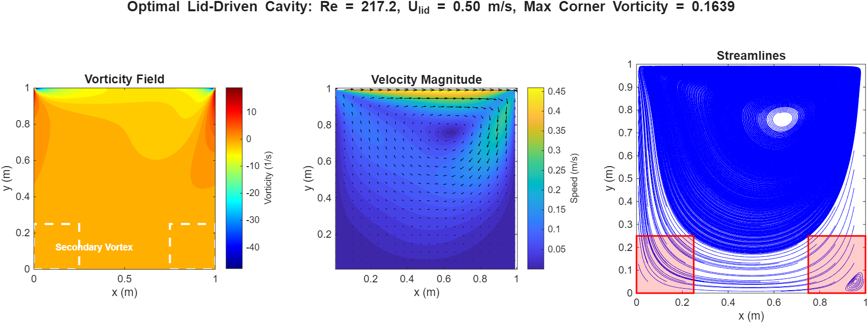
The fantastic thing about surrogateopt is that it builds a response floor because it goes. After simply 20 operate evaluations (about 5 minutes), it discovered the optimum working level—one thing that will have taken hours with a grid search.
What’s Subsequent?
The mix of MATLAB MCP Core Server + Optimization Toolbox opens up a complete new approach of doing engineering optimization. As a substitute of context-switching between documentation, code editor, and command window, you may have a dialog with an AI that:
- Checks your toolboxes to know what solvers can be found
- Formulates the issue based mostly in your pure language description
- Writes and runs the code in your native MATLAB
- Iterates on errors with out you copying and pasting
If you wish to do this your self, head over to the MATLAB MCP Core Server repository and comply with the setup directions. The server offers 5 core instruments—however mixed with the 100+ features in Optimization Toolbox, the probabilities are infinite.
Pleased optimizing! 
See Additionally
- Releasing the MATLAB MCP Core Server on GitHub
- Surrogate Optimization Documentation
- 2D Lid-Pushed Cavity Circulate Solver
Particular due to Michio Inoue for the cavity circulation solver.
var css=””; var head = doc.head || doc.getElementsByTagName(‘head’)[0], fashion = doc.createElement(‘fashion’); head.appendChild(fashion); fashion.kind=”textual content/css”; if (fashion.styleSheet){ fashion.styleSheet.cssText = css; } else { fashion.appendChild(doc.createTextNode(css)); }

