Small-Peak Suppression with the H-Maxima Remodel » Steve on Picture Processing with MATLAB

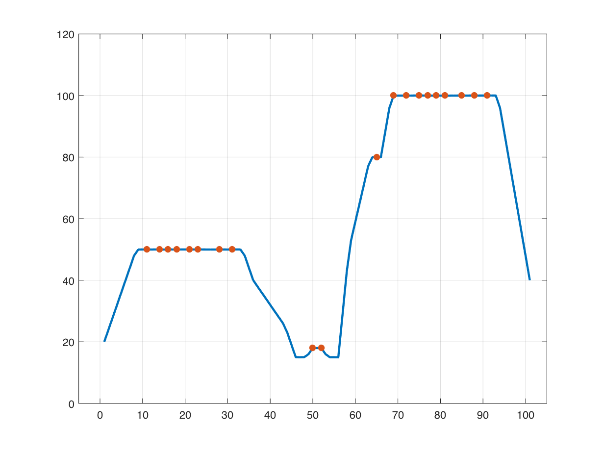
Let’s get there by beginning as soon as once more with the definition of regional most: a related element of pixels with a continuing worth h, the place each pixel that’s neighbor to that related element has a price that’s decrease than h. I would wish to elaborate on that utilizing a one-dimensional instance.

grid on

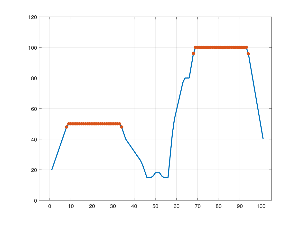
I am going to use dilation and erosion to establish curve samples which might be on plateaus.

plateau_mask = (y == imdilate(y,[1 1 1])) & (y == imerode(y,[1 1 1]));

plateau_mask = imdilate(plateau_mask,[1 1 1]);

plot(x(plateau_mask),y(plateau_mask),“*”)

maintain off

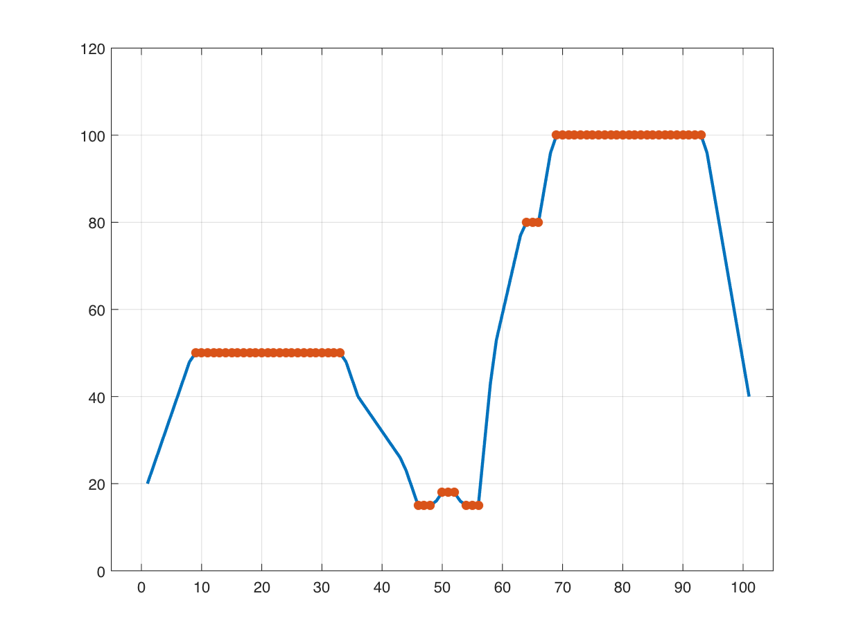
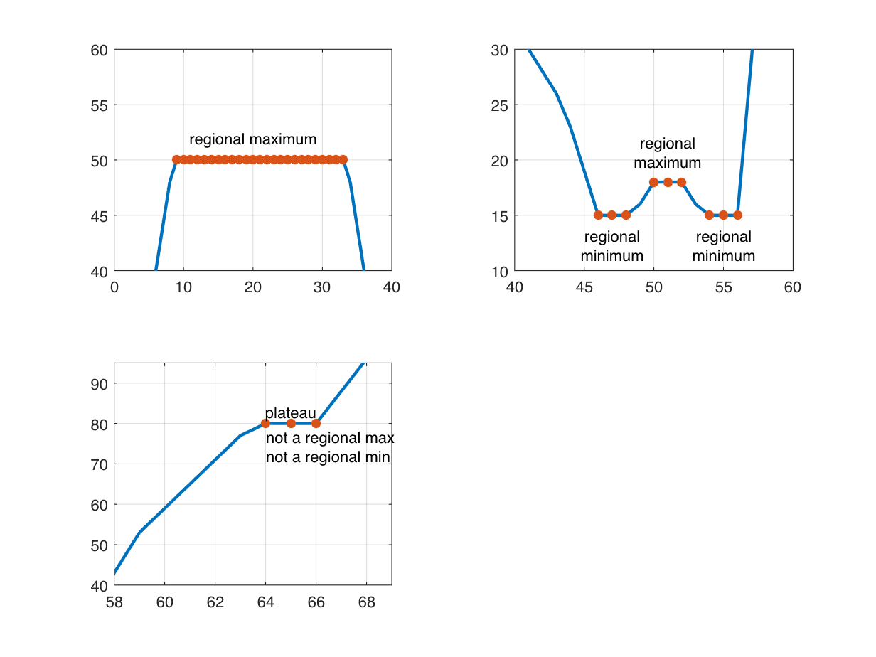
Listed below are some zoomed-in views that illustrate three sorts of plateaus which might be of curiosity.

plot(x(plateau_mask),y(plateau_mask),“*”)

textual content(20,52,“regional most”,HorizontalAlignment=“middle”)

plot(x(plateau_mask),y(plateau_mask),“*”)

textual content(47,14,[“regional” “minimum”],HorizontalAlignment = “middle”,…

VerticalAlignment = “prime”)

textual content(55,14,[“regional” “minimum”],HorizontalAlignment = “middle”,…

VerticalAlignment = “prime”)

textual content(51,19,[“regional” “maximum”],HorizontalAlignment = “middle”,…

VerticalAlignment = “backside”)

plot(x(plateau_mask),y(plateau_mask),“*”)

textual content(66,83,“plateau”,HorizontalAlignment = “proper”)

textual content(64,79,[“not a regional max” “not a regional min”],…

HorizontalAlignment = “left”, VerticalAlignment = “prime”)

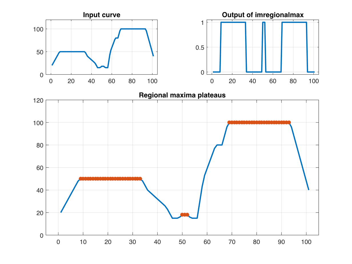
As I confirmed final time, the operate imregionalmax identifies the placement of regional maxima. These may be particular person samples or pixels, or they are often plateaus. Have a look:

reg_max_mask = imregionalmax(y);

axis([-5 105 -0.05 1.05])

title(“Output of imregionalmax”)

plot(x(reg_max_mask),y(reg_max_mask),“*”)

title(“Regional maxima plateaus”)

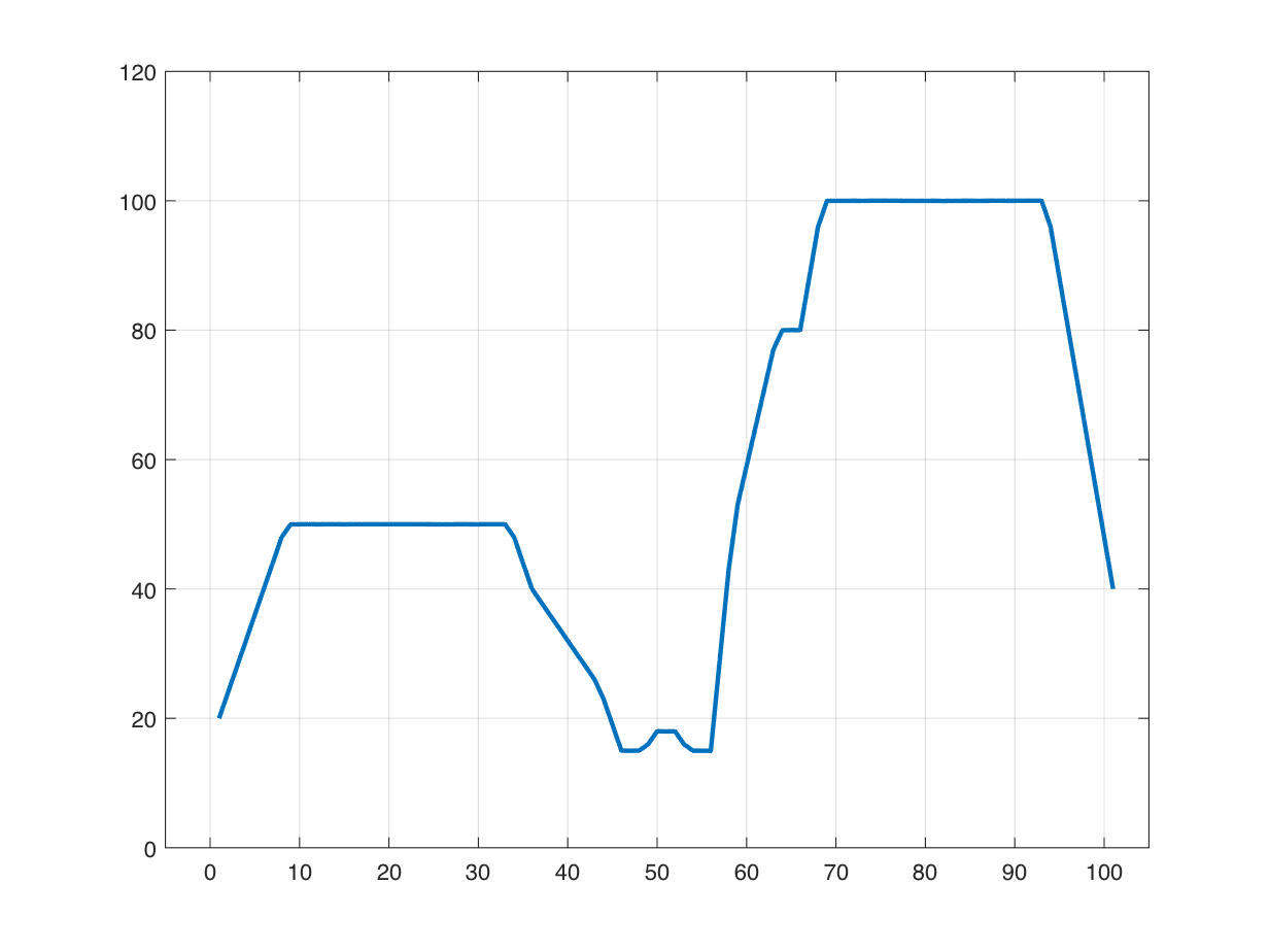
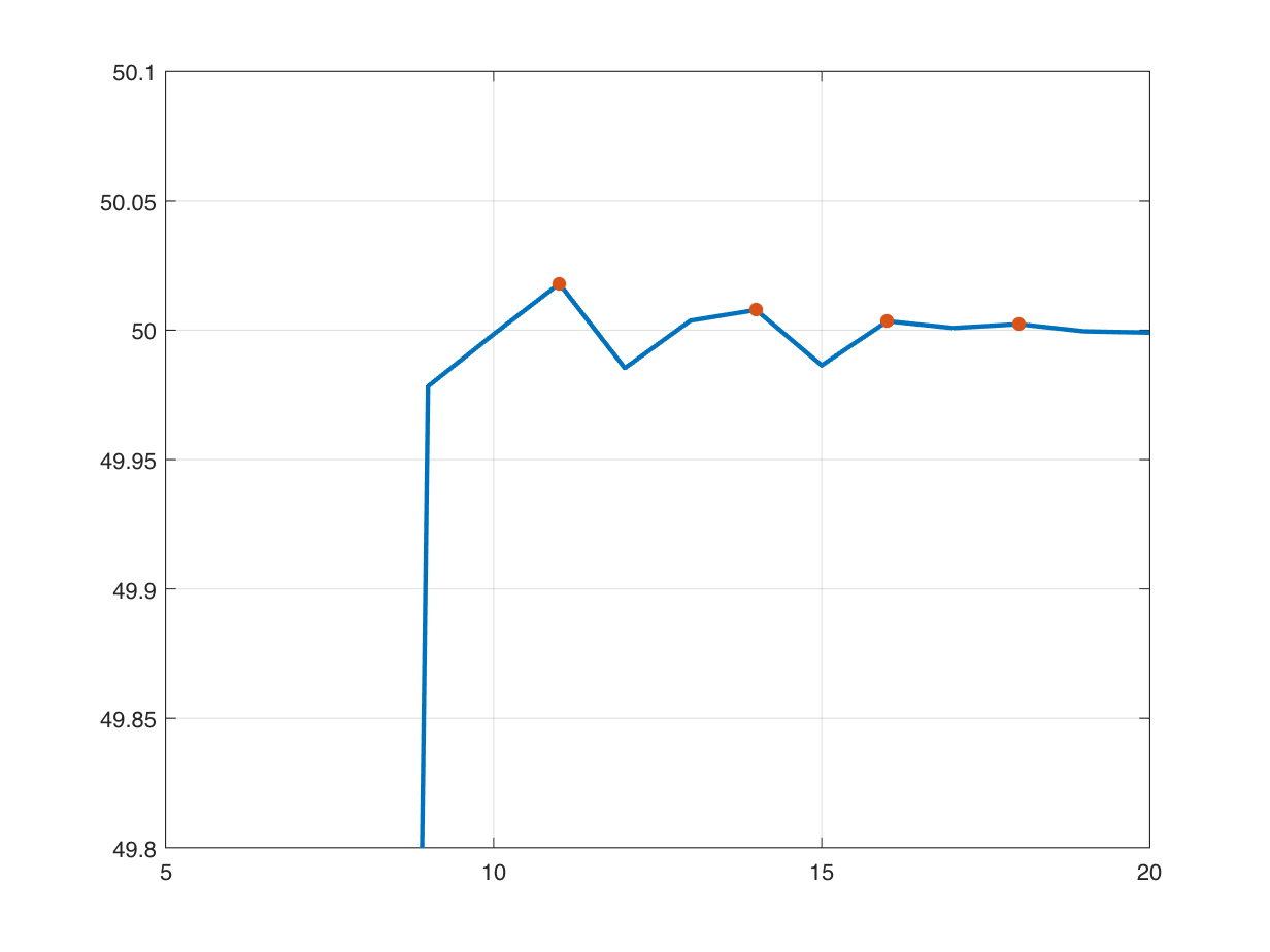
The curve I have been experimenting with is comparatively easy, with plateaus which might be fully flat. Sadly, the imregionalmax is considerably much less helpful when the enter is even a bit of noisy. That is as a result of noise introduces small native maxima in lots of locations, and imregionalmax picks up even the tiniest native maxima. Let’s attempt it. If I add a really small quantity of noise, you’ll be able to’t even see it within the plot:

yn = y + (0.01 * randn(dimension(y)));

grid on

However now the output of imregionalmax seems to be fully totally different.

reg_max_mask_n = imregionalmax(yn);

plot(x(reg_max_mask_n),yn(reg_max_mask_n),“*”)

grid on

Now, solely a scattering of samples on the broad plateaus are recognized as regional maxima, and a pattern on the small “shoulder” plateau is marked as a regional most the place it wasn’t earlier than. We’ve got to zoom in fairly far to see why that is taking place.

axis([5 20 49.8 50.1])

axis([62 67 79.9 80.2])

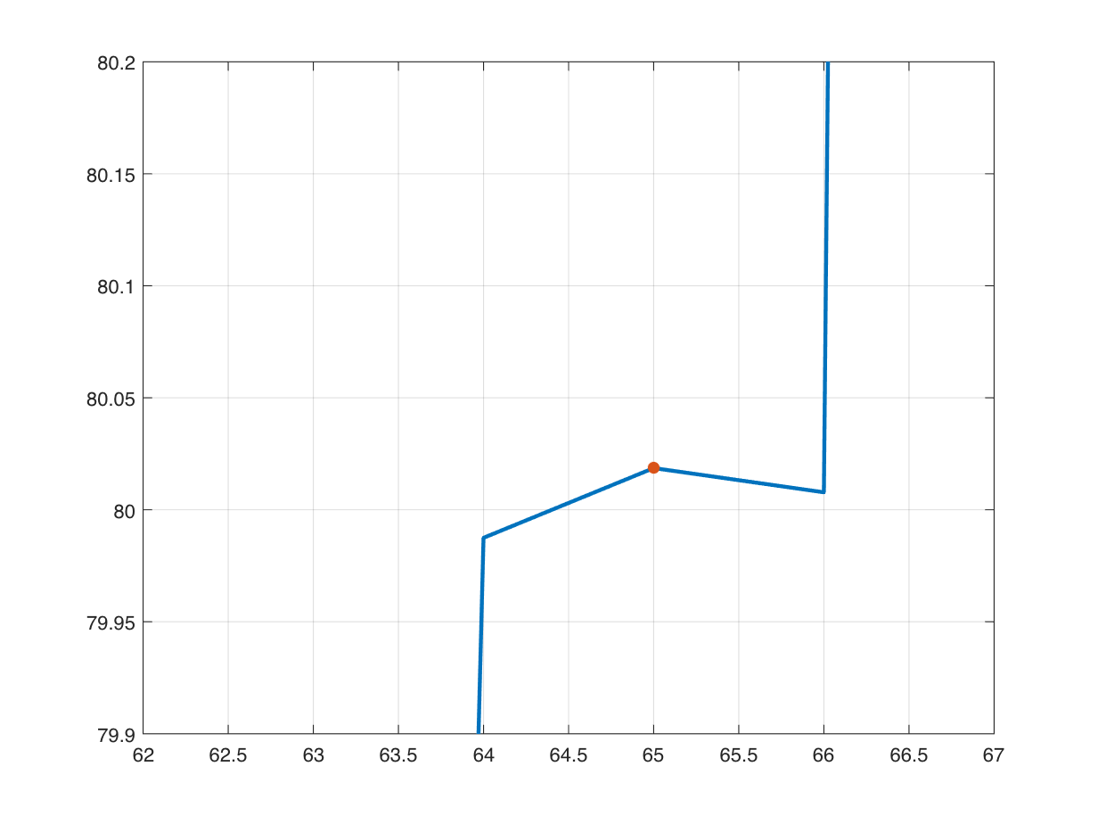
You may see that the added noise is introducing tiny native maxima in varied locations, and that’s throwing imregionalmax off the scent from what we might like for it to do.

imhmax

And this is the place the operate imhmax comes into play. It computes one thing referred to as the h-maxima rework. This operation basically suppresses any native maxima which might be lower than a sure top (h) above their rapid environment. As an instance, for instance, that we’re solely fascinated with native or regional maxima which have a top of greater than 5 models above their rapid environment. We accomplish this by calling imhmax like this:

legend([“original” “h-maxima transform”])

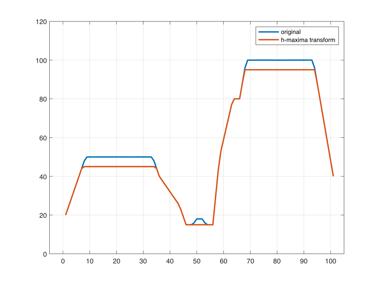
Within the output of imhmax, the broad peaks have been flattened out, and the small peak within the center, which has a top of solely 3 above its environment, has been flattened out and eradicated. Now let’s attempt imregionalmax once more.

reg_max_mask_n_h = imregionalmax(yn_h);

plot(x(reg_max_mask_n_h),yn(reg_max_mask_n_h),“*”)

grid on

With that computation, now we have recognized solely the peaks which might be considerably greater than what’s round them, and that is usually what we’re fascinated with. Discover that the h-maxima rework spreads out the height a bit, and so the end result proven above is selecting out a little bit of the “shoulders” to the left and proper of every broad plateau. We may do some post-processing to right that, if needed.

There may be one other operate, imextendedmax, that merely combines the h-maxima rework and regional maxima steps right into a single operate. Should you’re fascinated with minima as a substitute, then you should utilize the upside-down variations of those capabilities: imhmin, imregionalmin, and imextendedmin.

You probably have discovered fascinating makes use of for these capabilities in your personal work, I would love to listen to about it, so please depart a remark.

Utility operate