

Introduction
Thresholding is an easy and environment friendly method to carry out primary segmentation in a picture, and to binarize it (flip it right into a binary picture) the place pixels are both 0 or 1 (or 255 for those who’re utilizing integers to symbolize them).
Sometimes, you should utilize thresholding to carry out easy background-foreground segmentation in a picture, and it boils all the way down to variants on a easy method for every pixel:
if pixel_value > threshold:
    pixel_value = MAX
else:
    pixel_value = 0
This important course of is named Binary Thresholding. Now – there are numerous methods you possibly can tweak this common concept, together with inverting the operations (switching the > signal with a < signal), setting the pixel_value to the threshold as a substitute of a most worth/0 (often called truncating), preserving the pixel_value itself if it is above the threshold or if it is beneath the threshold.
All of those have conveniently been applied in OpenCV as:
cv2.THRESH_BINARYcv2.THRESH_BINARY_INVcv2.THRESH_TRUNCcv2.THRESH_TOZEROcv2.THRESH_TOZERO_INV
… respectively. These are comparatively “naive” strategies in that hey’re pretty easy, do not account for context in pictures, have information of what shapes are frequent, and so on. For these properties – we might should make use of far more computationally costly and highly effective strategies.
Now, even with the “naive” strategies – some heuristics may be put into place, for locating good thresholds, and these embrace the Otsu methodology and the Triangle methodology:
cv2.THRESH_OTSUcv2.THRESH_TRIANGLE
Notice: OpenCV thresholding is a rudimentary method, and is delicate to lighting adjustments and gradients, colour heterogeneity, and so on. It is best utilized on comparatively clear photos, after blurring them to scale back noise, with out a lot colour variance within the objects you need to phase.
One other method to overcome among the points with primary thresholding with a single threshold worth is to make use of adaptive thresholding which applies a threshold worth on every small area in a picture, quite than globally.
Easy Thresholding with OpenCV
Thresholding in OpenCV’s Python API is finished by way of the cv2.threshold() methodology – which accepts a picture (NumPy array, represented with integers), the brink, most worth and thresholding methodology (how the threshold and maximum_value are used):
img = cv2.imread('objects.jpg')

img = cv2.cvtColor(img, cv2.COLOR_BGR2RGB)


blurred = cv2.GaussianBlur(img, (7, 7), 0)

ret, img_masked = cv2.threshold(blurred, 220, 255, cv2.THRESH_BINARY)
The return code is simply the utilized threshold:
print(f"Threshold: {ret}")
Right here, because the threshold is 220 and we have used the THRESH_BINARY methodology – each pixel worth above 220 shall be elevated to 255, whereas each pixel worth beneath 220 shall be lowered to 0, making a black and white picture, with a “masks”, protecting the foreground objects.
Why 220? Realizing what the picture seems to be like means that you can make some approximate guesses about what threshold you possibly can select. In follow, you may not often need to set a handbook threshold, and we’ll cowl computerized threshold choice in a second.
Let’s plot the consequence! OpenCV home windows generally is a bit finicky, so we’ll plot the unique picture, blurred picture and outcomes utilizing Matplotlib:
fig, ax = plt.subplots(1, 3, figsize=(12, 8))
ax[0].imshow(img)
ax[1].imshow(blurred)
ax[2].imshow(img_masked)

Thresholding Strategies
As talked about earlier, there are numerous methods you should utilize the brink and most worth in a operate. We have taken a have a look at the binary threshold initially. Let’s create a listing of strategies, and apply them one after the other, plotting the outcomes:
strategies = [cv2.THRESH_BINARY, cv2.THRESH_BINARY_INV, cv2.THRESH_TRUNC, cv2.THRESH_TOZERO, cv2.THRESH_TOZERO_INV]
names = ['Binary Threshold', 'Inverse Binary Threshold', 'Truncated Threshold', 'To-Zero Threshold', 'Inverse To-Zero Threshold']

def thresh(img_path, methodology, index):
    img = cv2.imread(img_path)
    img = cv2.cvtColor(img, cv2.COLOR_BGR2RGB)
    blurred = cv2.GaussianBlur(img, (7, 7), 0)
    ret, img_masked = cv2.threshold(blurred, 220, 255, methodology)

    fig, ax = plt.subplots(1, 3, figsize=(12, 4))
    fig.suptitle(names[index], fontsize=18)
    ax[0].imshow(img)
    ax[1].imshow(blurred)
    ax[2].imshow(img_masked)
    plt.tight_layout()

for index, methodology in enumerate(strategies):
    thresh('cash.jpeg', methodology, index)
THRESH_BINARY and THRESH_BINARY_INV are inverse of one another, and binarize a picture between 0 and 255, assigning them to the background and foreground respectively, and vice versa.
THRESH_TRUNC binarizes the picture between threshold and 255.
THRESH_TOZERO and THRESH_TOZERO_INV binarize between 0 and the present pixel worth (src(x, y)). Let’s check out the ensuing pictures:

Try our hands-on, sensible information to studying Git, with best-practices, industry-accepted requirements, and included cheat sheet. Cease Googling Git instructions and really study it!


These strategies are intuitive sufficient – however, how can we automate a very good threshold worth, and what does a “good threshold” worth even imply? Many of the outcomes to date had non-ideal masks, with marks and specks in them. This occurs due to the distinction within the reflective surfaces of the cash – they are not uniformly coloured because of the distinction in how ridges replicate gentle.
We will, to a level, battle this by discovering a greater world threshold.
Automated/Optimized Thresholding with OpenCV
OpenCV employs two efficient world threshold looking out strategies – Otsu’s methodology, and the Triangle methodology.
Otsu’s methodology assumes that it is engaged on bi-modal pictures. Bi-modal pictures are pictures whose colour histograms solely include two peaks (i.e. has solely two distinct pixel values). Contemplating that the peaks every belong to a category reminiscent of a “background” and “foreground” – the best threshold is true in the course of them.
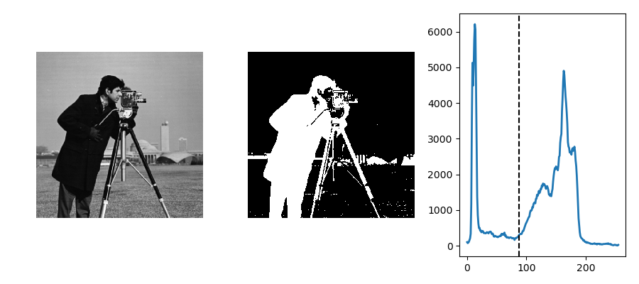
Picture credit score: https://scipy-lectures.org/
You may make some pictures extra bi-modal with gaussian blurs, however not all.
Another, oftentimes higher performing algorithm is the triangle algorithm, which calculates the gap between the utmost and minimal of the grey-level histogram and attracts a line. The purpose at which that line is maximally far-off from the remainder of the histogram is chosen because the treshold:

Each of those assume a greyscaled picture, so we’ll have to convert the enter picture to grey by way of cv2.cvtColor():
img = cv2.imread(img_path)
grey = cv2.cvtColor(img, cv2.COLOR_BGR2GRAY)
blurred = cv2.GaussianBlur(grey, (7, 7), 0)

ret, mask1 = cv2.threshold(blurred, 0, 255, cv2.THRESH_OTSU)
ret, mask2 = cv2.threshold(blurred, 0, 255, cv2.THRESH_TRIANGLE)

masked = cv2.bitwise_and(img, img, masks=mask1)
Let’s run the picture via with each strategies and visualize the outcomes:
strategies = [cv2.THRESH_OTSU, cv2.THRESH_TRIANGLE]
names = ['Otsu Method', 'Triangle Method']

def thresh(img_path, methodology, index):
    img = cv2.imread(img_path)
    grey = cv2.cvtColor(img, cv2.COLOR_BGR2GRAY)
    blurred = cv2.GaussianBlur(grey, (7, 7), 0)

    ret, img_masked = cv2.threshold(blurred, 0, 255, methodology)
    print(f"Threshold: {ret}")

    fig, ax = plt.subplots(1, 3, figsize=(12, 5))
    fig.suptitle(names[index], fontsize=18)
    ax[0].imshow(cv2.cvtColor(img, cv2.COLOR_BGR2RGB))
    ax[1].imshow(cv2.cvtColor(grey, cv2.COLOR_BGR2RGB))
    ax[2].imshow(cv2.cvtColor(img_masked, cv2.COLOR_BGR2RGB))

for index, methodology in enumerate(strategies):
    thresh('cash.jpeg', methodology, index)
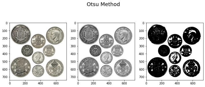
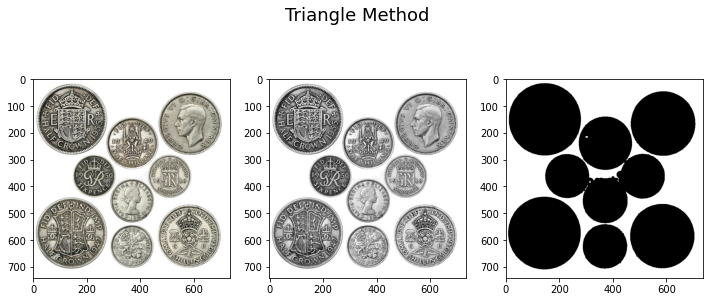
Right here, the triangle methodology outperforms Otsu’s methodology, as a result of the picture is not bi-modal:
import numpy as np

img = cv2.imread('cash.jpeg')
grey = cv2.cvtColor(img, cv2.COLOR_BGR2GRAY)
blurred = cv2.GaussianBlur(grey, (7, 7), 0)

histogram_gray, bin_edges_gray = np.histogram(grey, bins=256, vary=(0, 255))
histogram_blurred, bin_edges_blurred = np.histogram(blurred, bins=256, vary=(0, 255))

fig, ax = plt.subplots(1, 2, figsize=(12, 4))

ax[0].plot(bin_edges_gray[0:-1], histogram_gray)
ax[1].plot(bin_edges_blurred[0:-1], histogram_blurred)

Nonetheless, it is clear how the triangle methodology was capable of work with the picture and produce a extra satisfying consequence.
Limitations of OpenCV Thresholding
Thresholding with OpenCV is straightforward, simple and environment friendly. But, it is pretty restricted. As quickly as you introduce colourful components, non-uniform backgrounds and altering lighting situations – world thresholding as an idea turns into too inflexible.
Photos are often too complicated for a single threshold to be sufficient, and this may partially be addressed via adaptive thresholding, the place many native thresholds are utilized as a substitute of a single world one. Whereas additionally restricted, adaptive thresholding is far more versatile than world thresholding.
Conclusion
In recent times, binary segmentation (like what we did right here) and multi-label segmentation (the place you possibly can have an arbitrary variety of lessons encoded) has been efficiently modeled with deep studying networks, that are far more highly effective and versatile. As well as, they’ll encode world and native context into the pictures they’re segmenting. The draw back is – you want knowledge to coach them, in addition to time and experience.
For on-the-fly, easy thresholding, you should utilize OpenCV. For correct, production-level segmentation, you may need to use neural networks.
Going Additional – Sensible Deep Studying for Laptop Imaginative and prescient
Your inquisitive nature makes you need to go additional? We suggest testing our Course: “Sensible Deep Studying for Laptop Imaginative and prescient with Python”.

One other Laptop Imaginative and prescient Course?
We cannot be doing classification of MNIST digits or MNIST vogue. They served their half a very long time in the past. Too many studying sources are specializing in primary datasets and primary architectures earlier than letting superior black-box architectures shoulder the burden of efficiency.
We need to concentrate on demystification, practicality, understanding, instinct and actual tasks. Need to study how you can also make a distinction? We’ll take you on a trip from the best way our brains course of pictures to writing a research-grade deep studying classifier for breast most cancers to deep studying networks that “hallucinate”, instructing you the rules and concept via sensible work, equipping you with the know-how and instruments to change into an skilled at making use of deep studying to unravel pc imaginative and prescient.
What’s inside?
- The primary rules of imaginative and prescient and the way computer systems may be taught to “see”
- Totally different duties and purposes of pc imaginative and prescient
- The instruments of the commerce that may make your work simpler
- Discovering, creating and using datasets for pc imaginative and prescient
- The idea and utility of Convolutional Neural Networks
- Dealing with area shift, co-occurrence, and different biases in datasets
- Switch Studying and using others’ coaching time and computational sources to your profit
- Constructing and coaching a state-of-the-art breast most cancers classifier
- Methods to apply a wholesome dose of skepticism to mainstream concepts and perceive the implications of broadly adopted strategies
- Visualizing a ConvNet’s “idea house” utilizing t-SNE and PCA
- Case research of how firms use pc imaginative and prescient strategies to realize higher outcomes
- Correct mannequin analysis, latent house visualization and figuring out the mannequin’s consideration
- Performing area analysis, processing your individual datasets and establishing mannequin assessments
- Reducing-edge architectures, the development of concepts, what makes them distinctive and find out how to implement them
- KerasCV – a WIP library for creating state-of-the-art pipelines and fashions
- Methods to parse and browse papers and implement them your self
- Choosing fashions relying in your utility
- Creating an end-to-end machine studying pipeline
- Panorama and instinct on object detection with Sooner R-CNNs, RetinaNets, SSDs and YOLO
- Occasion and semantic segmentation
- Actual-Time Object Recognition with YOLOv5
- Coaching YOLOv5 Object Detectors
- Working with Transformers utilizing KerasNLP (industry-strength WIP library)
- Integrating Transformers with ConvNets to generate captions of pictures
- DeepDream
- Deep Studying mannequin optimization for pc imaginative and prescient