

We are able to tighten the evaluation of gradient descent with momentum by a cobination of Chebyshev polynomials of the primary and second form. Following this connection, we’ll derive one of the crucial iconic strategies in optimization: Polyak momentum.
$$
defaa{boldsymbol a}
defrr{boldsymbol r}
defAA{boldsymbol A}
defHH{boldsymbol H}
defEE{mathbb E}
defII{boldsymbol I}
defCC{boldsymbol C}
defDD{boldsymbol D}
defKK{boldsymbol Okay}
defeeps{boldsymbol varepsilon}
deftr{textual content{tr}}
defLLambda{boldsymbol Lambda}
defbb{boldsymbol b}
defcc{boldsymbol c}
defxx{boldsymbol x}
defzz{boldsymbol z}
defuu{boldsymbol u}
defvv{boldsymbol v}
defqq{boldsymbol q}
defyy{boldsymbol y}
defss{boldsymbol s}
defpp{boldsymbol p}
deflmax{L}
deflmin{mu}
defRR{mathbb{R}}
defTT{boldsymbol T}
defQQ{boldsymbol Q}
defCC{boldsymbol C}
defEcond{boldsymbol E}
DeclareMathOperator*{argmin}{{arg,min}}
DeclareMathOperator*{argmax}{{arg,max}}
DeclareMathOperator*{decrease}{{decrease}}
DeclareMathOperator*{dom}{mathbf{dom}}
DeclareMathOperator*{Repair}{mathbf{Repair}}
DeclareMathOperator{prox}{mathbf{prox}}
DeclareMathOperator{span}{mathbf{span}}
defdefas{stackrel{textual content{def}}{=}}
defdif{mathop{}!mathrm{d}}
definecolor{colormomentum}{RGB}{27, 158, 119}
definecolor{colorstepsize}{RGB}{217, 95, 2}
$$
Gradient Descent with Momentum
Gradient descent with momentum, often known as heavy ball or momentum for brief, is an optimization
technique
designed to resolve unconstrained optimization issues of the shape
start{equation}
argmin_{xx in RR^d} f(xx),,
finish{equation}
the place the target perform $f$ is differentiable and we’ve got entry to its gradient $nabla
f$. On this technique
the udpate is a sum of two phrases. The primary time period is the
distinction between present and former iterate $(xx_{t} – xx_{t-1})$, often known as momentum
time period. The second time period is the gradient $nabla f(xx_t)$ of the target perform.
Gradient Descent with Momentum
Enter: beginning guess $xx_0$, step-size ${coloration{colorstepsize} h} > 0$ and momentum
parameter ${coloration{colormomentum} m} in (0, 1)$.
$xx_1 = xx_0 – dfrac{{coloration{colorstepsize} h}}{1 + {coloration{colormomentum} m}} nabla f(xx_0)$
For $t=1, 2, ldots$ compute
start{equation}label{eq:momentum_update}
xx_{t+1} = xx_t + {coloration{colormomentum} m}(xx_{t} – xx_{t-1}) – {coloration{colorstepsize}
h}nabla
f(xx_t)
finish{equation}
Gradient descent with momentum has seen a renewed curiosity lately, as a stochastic variant that replaces the true gradient with a stochastic estimate has proven to be very efficient for deep studying.
Quadratic mannequin
Though momentum will be utilized to any downside with a twice differentiable goal, on this submit we’ll assume for simplicity the target perform $f$ quadratic.
As within the earlier submit, we’ll assume the target is
start{equation}label{eq:decide}
f(xx) defas frac{1}{2}xx^prime HH xx + bb^prime xx~,
finish{equation}
the place $HH$ is a optimistic particular sq. matrix with eigenvalues within the interval $[lmin, L]$.
Instance: Polyak Momentum, often known as the HeavyBall technique, is a extensively used occasion of momentum. Initially developed for the answer of linear equations and referred to as Frankel’s technique,
Boris Polyak (1935 —) is a Russian mathematician and pioneer of optimization. At the moment, he leads the Laboratory at Institute of Management Science in Moscow.
Polyak momentum follows the replace eqref{eq:momentum_update} with momentum and step-size parameters
start{equation}label{eq:polyak_parameters}
{coloration{colormomentum}m = {Huge(frac{sqrt{L}-sqrt{lmin}}{sqrt{L}+sqrt{lmin}}Huge)^2}}
textual content{ and }
{coloration{colorstepsize}h = Huge(frac{ 2}{sqrt{L}+sqrt{lmin}}Huge)^2},,
finish{equation}
which supplies the complete algorithm
Polyak Momentum
Enter: beginning guess $xx_0$, decrease and higher eigenvalue certain $lmin$ and $L$.
$xx_1 = xx_0 – {coloration{colorstepsize}frac{2}{L + lmin}} nabla f(xx_0)$
For $t=1, 2, ldots$ compute
start{equation}label{eq:polyak_momentum_update}
xx_{t+1} = xx_t + {coloration{colormomentum} {Huge(tfrac{sqrt{L}-sqrt{lmin}}{sqrt{L}+sqrt{lmin}}Huge)^2}}(xx_{t} – xx_{t-1}) – {coloration{colorstepsize} Huge(tfrac{ 2}{sqrt{L}+sqrt{lmin}}Huge)^2}nabla
f(xx_t)
finish{equation}
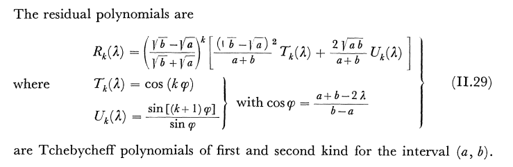
Residual Polynomials
Within the final submit we noticed that to every gradient-based optimizer we will affiliate a sequence of
polynomials $P_1, P_2,
…$ that we named residual polynomials and that determines the converge of the tactic:
the sequence of
residual polynomials related to this technique. Then the error at every iteration $t$ verifies
start{equation}
xx_t – xx^star = P_t(HH)(xx_0 – xx^star),.
finish{equation}
This can be a particular case of the Residual polynomial Lemma proved within the final submit.
Within the final submit we additionally gave an expression for this residual polynomial. Though this expression is moderately concerned within the common case, it simplifies for momentum, the place it follows the straightforward recurrence:
Given a momentum technique with parameters
${coloration{colormomentum} m}$, ${coloration{colorstepsize}
h}$, the related residual polynomials $P_0, P_1, ldots$ confirm the next recursion
start{equation}
start{break up}
&P_{t+1}(lambda) = (1 + {coloration{colormomentum}m} – {coloration{colorstepsize} h} lambda ) P_{t}(lambda) –
{coloration{colormomentum}m} P_{t-1}(lambda)
&P_0(lambda) = 1,,~ P_1(lambda) = 1 – frac{{coloration{colorstepsize} h}}{1 + {coloration{colormomentum}m}} lambda ,.
finish{break up}label{eq:def_residual_polynomial2}
finish{equation}
A consequence of this result’s that not solely the tactic, but additionally its residual polynomial, has a easy recurrence. We’ll quickly leverage this to simplify the evaluation.
Chebyshev meets Chebyshev
Chebyshev polynomials of the primary form appeared within the final submit when deriving the optimum worst-case technique. These are polynomials
$T_0, T_1, ldots$ outlined by the recurrence relation
start{align}
&T_0(lambda) = 1 qquad T_1(lambda) = lambda
&T_{okay+1}(lambda) = 2 lambda T_k(lambda) – T_{k-1}(lambda)~.
finish{align}
A undeniable fact that we did not use within the final submit is that Chebyshev polynomials are orthogonal with respect to the burden perform
start{equation}
difomega(lambda) = start{instances} frac{1}{pisqrt{1 – lambda^2}} &textual content{ if $lambda in
[-1, 1]$} 0 &textual content{ in any other case},. finish{instances}
finish{equation}
That’s, they confirm the orthogonality situation
start{equation}
int T_i(lambda) T_j(lambda) difomega(lambda) start{instances} > 0 textual content{ if $i = j$} = 0
textual content{ in any other case},.finish{instances}
finish{equation}
I discussed that these are the Chebyshev polynomials of the primary form as a result of there are
additionally Chebyshev polynomials of the second form, and though much less used, additionally of the third
form, fourth form and so forth.
Chebyshev polynomials of the second form, denoted $U_1, U_2, ldots$, are outlined by the
integral
start{equation}
U_t(lambda) = int frac{T_{t+1}(xi) – T_{t+1}(lambda)}{xi- lambda}difomega(xi),.
finish{equation}
Though we are going to solely use this development for Chebyshev polynomials, it extends past this
setup and may be very pure as a result of these polynomials are the numerators for the convergents of
sure continued fractions.
The polynomials of the second form confirm the identical recurrence components as the unique sequence,
however with completely different preliminary situations. Particularly, the Chebyshev polynomials of the second
form are decided by the recurrence
start{align}
&U_0(lambda) = 1 qquad U_1(lambda) = 2 lambda
&U_{okay+1}(lambda) = 2 lambda U_k(lambda) – U_{k-1}(lambda)~.
finish{align}
Word how $U_1(lambda)$ is completely different from $T_1$, however aside from that, the coefficients within the
recurrence are the identical. Due to this, each sequences behave considerably equally, but additionally have essential variations. For instance, each varieties have extrema on the endpoints, however the worth is completely different. For the primary form, the
extrema is $pm 1$, whereas for the second form its $pm (t+1)$.
Picture of the primary 6 Chebyshev polynomials of the primary and second
form within the $[-1, 1]$ interval.
![]()


Momentum’s residual polynomial
Time has lastly come for the primary end result: the residual polynomial of
gradient descent with momentum is nothing else than a mix of Chebyshev polynomials of the primary and second
form. Because the properties of Chebyshev polynomials are well-known, this may present a approach to derive convergence bounds for momentum.
Contemplate the momentum technique with step-size ${coloration{colorstepsize}h}$ and momentum parameter ${coloration{colormomentum}m}$.
The residual polynomial $P_t$ related to this technique
will be written by way of Chebyshev
polynomials as
start{equation}label{eq:theorem}
P_t(lambda) = {coloration{colormomentum}m}^{t/2} left( {smallfrac{2
{coloration{colormomentum}m}}{1 + {coloration{colormomentum}m}}},
T_t(sigma(lambda))
+ {smallfrac{1 – {coloration{colormomentum}m}}{1 + {coloration{colormomentum}m}}},
U_t(sigma(lambda))proper),,
finish{equation}
with $sigma(lambda) = {smalldfrac{1}{2sqrt{{coloration{colormomentum}m}}}}(1 +
{coloration{colormomentum}m} –
{coloration{colorstepsize} h},lambda),$.
Let’s denote by $widetilde{P}_t$ the fitting hand aspect of the above equation, that’s,
start{equation}
widetilde{P}_{t}(lambda) defas {coloration{colormomentum}m}^{t/2} left( {smallfrac{2
{coloration{colormomentum}m}}{1 + {coloration{colormomentum}m}}},
T_t(sigma(lambda))
+ {smallfrac{1 – {coloration{colormomentum}m}}{1 + {coloration{colormomentum}m}}},
U_t(sigma(lambda))proper),.
finish{equation}
Our objective is to indicate that $P_t = widetilde{P}_t$ for all $t$.
For $t=1$, $T_1(lambda) = lambda$ and $U_1(lambda) = 2lambda$, so we’ve got
start{align}
widetilde{P}_1(lambda) &= sqrt{{coloration{colormomentum}m}} left(tfrac{2
{coloration{colormomentum}m}}{1 + {coloration{colormomentum}m}} sigma(lambda) + tfrac{1 – {coloration{colormomentum}m}}{1 + {coloration{colormomentum}m}} 2
sigma(lambda)proper)
&= frac{2 sqrt{{coloration{colormomentum}m}}}{1 + {coloration{colormomentum}m}} sigma(lambda) = 1 – frac{{coloration{colorstepsize}h}}{1 + {coloration{colormomentum}m}} lambda,,
finish{align}
which corresponds to the definition of $P_1$ in eqref{eq:def_residual_polynomial2}.
Assume it is true for any iteration as much as $t$, we are going to present it is true for $t+1$. Utilizing the three-term recurrence of Chebyshev polynomials we’ve got
start{align}
&widetilde{P}_{t+1}(lambda) = {coloration{colormomentum}m}^{(t+1)/2} left( {smallfrac{2 {coloration{colormomentum}m}}{1 + {coloration{colormomentum}m}}},
T_{t+1}(sigma(lambda))
+ {smallfrac{1 – {coloration{colormomentum}m}}{1 + {coloration{colormomentum}m}}}, U_{t+1}(sigma(lambda))proper)
&= {coloration{colormomentum}m}^{(t+1)/2} Huge( {smallfrac{2
{coloration{colormomentum}m}}{1 + {coloration{colormomentum}m}}},
(2 sigma(lambda) T_{t}(sigma(lambda)) – T_{t-1}(sigma(lambda))) nonumber
&qquadqquad
+ {smallfrac{1 – {coloration{colormomentum}m}}{1 + {coloration{colormomentum}m}}}, (2 sigma(lambda)
U_{t}(sigma(lambda)) – U_{t-1}(sigma(lambda)))Huge)
&= 2 sigma(lambda) sqrt{{coloration{colormomentum}m}} P_t(lambda) – {coloration{colormomentum}m} P_{t-1}(lambda)
&= (1 + {coloration{colormomentum}m} – {coloration{colorstepsize}h} lambda) P_t(lambda) –
{coloration{colormomentum}m} P_{t-1}(lambda)
finish{align}
the place the third identification follows from grouping polynomials of identical diploma and the
induction speculation. The final expression is the recursive definition of $P_{t+1}$ in
eqref{eq:def_residual_polynomial2}, which proves the specified $widetilde{P}_{t+1} =
{P}_{t+1}$.
Historical past bits. The concept above is a generalization
Rutishauser in his 1959 e book.
identifies the residual polynomial comparable to Frankel’s technique (equal to Polyak
momentum on quadratic capabilities).
Extra just lately, in a collaboration with Courtney, Bart and Elliot we used Ruthishauser’s expression to derive an average-case evaluation of Polyak momentum.
Convergence Charges and Strong Area
Within the final submit se launched the worst-case
convergence charge as a device to match pace of convergence of optimization algorithms.
These are an higher certain on the per-iteration progress of an optimization algorithm. In different
phrases, a small convergence charge ensures a quick convergence. Convergence charges will be
expressed in time period of the residual polynomial as
start{equation}
r_t defas max_{lambda in [lmin, L]} |P_t(lambda)|,,
finish{equation}
the place $lmin, L$ are the smallest and largest eigenvalues of $HH$ respectively. Utilizing Hestenes and Stiefel’s lemma, we will see that $r_t$ is an higher certain on the norm of the error within the sense that it verifies
start{equation}
|xx_t – xx^star| leq r_t,|xx_0 – xx^star|,.
finish{equation}
Deriving convergence charges is tough, however the earlier Theorem permits us to transform this downside into the one in all bounding Chebyshev polynomials. Hopefully, this downside is simpler as we all know lots about Chebyshev polynomials. Particularly, changing $P_t$ with eqref{eq:theorem} within the definition of convergence charge and higher bounding the joint most with a separate one on $T_t$ and $U_t$ we’ve got
start{equation}
r_t leq {coloration{colormomentum}m}^{t/2} left( {smallfrac{2
{coloration{colormomentum}m}}{1 + {coloration{colormomentum}m}}},
max_{lambda in [lmin, L]}|T_t(sigma(lambda))|
+ {smallfrac{1 – {coloration{colormomentum}m}}{1 + {coloration{colormomentum}m}}}, max_{lambda in
[lmin, L]}|U_t(sigma(lambda))|proper),.
finish{equation}
On this equation we all know every little thing besides $max_{lambda in [lmin, L]}|T_t(sigma(lambda))|$
and $max_{lambda in [lmin, L]}|U_t(sigma(lambda))|$.
Fortunately, we’ve got all types of bounds on Chebyshev polynomials. One of many easiest and most
helpful one bounds these polynomials within the $[-1, 1]$ interval.
This interval (shaded blue area in left plot) accommodates all of the zeros of each polynomials, they usually’re bounded both by a relentless or by a time period that scales linearly with the iteration (Eq. eqref{eq:bound_chebyshev}).
Outdoors of this interval, each polynomials develop at a charge that’s exponential within the variety of iterations.
![]()
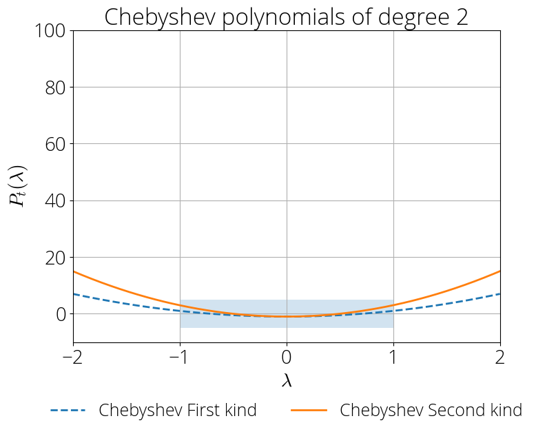
Contained in the interval $xi in [-1, 1]$, we’ve got the
bounds
start{equation}label{eq:bound_chebyshev}
|T_t(xi)| leq 1 quad textual content{ and } quad |U_{t}(xi)| leq t+1,.
finish{equation}
In our case, the Chebyshev polynomials are evaluated at $sigma(lambda)$, so these bounds are
legitimate each time $max_{lambda in [lmin, L]}|sigma(lambda)| leq 1$. Since $sigma$ is a linear perform of $lambda$, its extremal factors are reached on the edges of the interval, and so the earlier situation is equal to $|sigma(lmin)| leq 1 $ and $|sigma(L)| leq 1$, which reordering provides the situations
start{equation}label{eq:condition_stable_region}
frac{(1 – sqrt{{coloration{colormomentum}m}})^2 }{{coloration{colorstepsize}h}} leq lmin quad textual content{ and }quad L
leq~frac{(1 + sqrt{{coloration{colormomentum}m}})^2 }{{coloration{colorstepsize}h}},.
finish{equation}
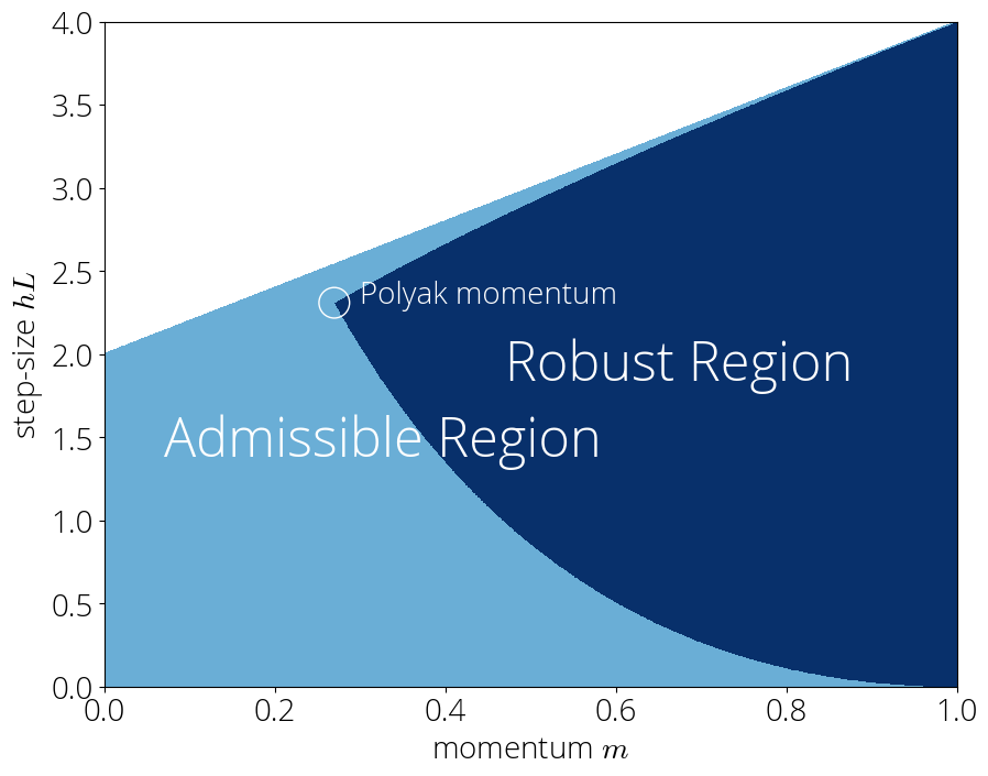
We’ll discuss with the set of parameters that
confirm the above because the strong area. This can be a subset of the set of admissible parameters –that’s, these for which the tactic converges–. The set of admissible parameters is
0 leq {coloration{colormomentum}m} lt 1 quad textual content{ and }quad {coloration{colorstepsize}h} lt frac{2 (1 + {coloration{colormomentum}m})}{L},.
finish{equation}
The strong area is the set of momentum (${coloration{colormomentum}m}$) and step-size parameters
(${coloration{colorstepsize}h}$) that fulfill inequality eqref{eq:condition_stable_region}. It is a subset of the set of parameters for which momentum converges (admissible area).
Instance of sturdy area for $lmin=0.1, L=1$.
![]()
Within the strong area, can use the bounds above and we’ve got the speed
start{equation}label{eq:convergence_rate_stable}
r_t leq {coloration{colormomentum}m}^{t/2} left( 1
+ {smallfrac{1 – {coloration{colormomentum}m}}{1 + {coloration{colormomentum}m}}}, tright)
finish{equation}
This convergence charge is considerably shocking, as one would possibly count on
that the convergence is dependent upon each the step-size and momentum. As a substitute, within the strong area the convergence charge
doesn’t rely upon the step-size. This
insensitivity to step-size will be leveraged for instance to develop a momentum tuner.
Provided that we want the convergence charge to be as small as doable, it is pure to decide on
the momentum time period as small as doable whereas staying within the strong area. However simply how small
can we make this momentum time period?
Polyak strikes again
This submit ends because it begins: with Polyak momentum. We’ll see that minimizing the convergence
charge whereas staying within the strong area will lead us naturally to this technique.
Contemplate the inequalities that describe the strong area:
start{equation}label{eq:robust_region_2}
frac{(1 – sqrt{{coloration{colormomentum}m}})^2 }{{coloration{colorstepsize}h}} leq lmin quad textual content{ and }quad L
leq~frac{(1 + sqrt{{coloration{colormomentum}m}})^2 }{{coloration{colorstepsize}h}},.
finish{equation}
Fixing for ${coloration{colorstepsize}h}$ on each equations permits us to explain the admissible values of ${coloration{colormomentum}m}$ as a single inequality:
start{equation}
left(frac{1 – sqrt{{coloration{colormomentum}m}} }{1 + sqrt{{coloration{colormomentum}m}}}proper)^2 leq lmin L,.
finish{equation}
The left hand aspect is monotonicallydecreasing in ${coloration{colormomentum}m}$. Since our goal is to decrease ${coloration{colormomentum}m}$, this shall be achieved when the inequality turns into an equality, which supplies
start{equation}
{coloration{colormomentum}m = {Huge(frac{sqrt{L}-sqrt{lmin}}{sqrt{L}+sqrt{lmin}}Huge)^2}}
finish{equation}
Lastly, the step-size parameter ${coloration{colorstepsize}h}$ will be computed from plugging the above momentum parameter into both one of many inequalities eqref{eq:robust_region_2}:
start{equation}
{coloration{colorstepsize}h = Huge(frac{ 2}{sqrt{L}+sqrt{lmin}}Huge)^2},.
finish{equation}
These are the step-size and momentum parameter of Polyak momentum of eqref{eq:polyak_parameters}.
This supplies an alternate derivation of Polyak momentum from Chebyshev polynomials.
consists in taking the restrict $tto infty$ of the Chebyshev iterative technique derived in
the earlier submit. See as an example paragraph “Less complicated stationary recursion” in Francis’ weblog submit.
convergence charge without cost. Since this mix of step-size and momentum belongs to the
strong area, we will apply eqref{eq:convergence_rate_stable}, which supplies
start{align}
r_t^{textual content{Polyak}} &leq left({smallfrac{sqrt{L} – sqrt{lmin}}{sqrt{L} +
sqrt{lmin}}}proper)^tleft({small 1 + tfrac{2 sqrt{L lmin}}{L + lmin}}proper)
label{eq:nonasymptotic_polyak},.
finish{align}
This suggests that the convergence charge of Polyak momentum –because the Chebyshev technique– is asymptotically bounded as
start{equation}
limsup_{t to infty} sqrt[t]{r_t^{textual content{Polyak}}} leq {smallfrac{sqrt{L} – sqrt{lmin}}{sqrt{L} +
sqrt{lmin}}},,
finish{equation}
which is a whopping sq. root
issue enchancment over gradient descent’s $frac{lmax – lmin}{lmax +
lmin}$ convergence charge charge.
Keep Tuned
On this submit we have solely scratched the floor of the wealthy dynamics of momentum.
Within the subsequent submit we are going to discover dig deeper into the strong area and discover the opposite areas too.
Citing
For those who discover this weblog submit helpful, please contemplate citing it as:
Momentum: when Chebyshev meets Chebyshev., Fabian Pedregosa, 2020
Bibtex entry:
    @misc{pedregosa2021residual,
      title={Momentum: when Chebyshev meets Chebyshev},
      creator={Pedregosa, Fabian},
      url = {http://fa.bianp.internet/weblog/2020/momentum/},
      yr={2020}
    }
Acknowledgements. Because of Baptiste Goujaud for reporting many typos and making glorious clarifying solutions, and to
Nicolas Le Roux for catching some errors in an preliminary model of this submit and offering considerate suggestions.