

Backtracking step-size methods (also referred to as adaptive step-size or approximate line-search) that set the step-size based mostly on a adequate lower situation are the usual method to set the step-size on gradient descent and quasi-Newton strategies. Nonetheless, these methods are a lot much less widespread for Frank-Wolfe-like algorithms. On this weblog publish I talk about a backtracking line-search for the Frank-Wolfe algorithm.
$$
defaa{boldsymbol a}
defbb{boldsymbol b}
defdd{boldsymbol d}
defcc{boldsymbol c}
defxx{boldsymbol x}
defzz{boldsymbol z}
defuu{boldsymbol u}
defvv{boldsymbol v}
defyy{boldsymbol y}
defss{boldsymbol s}
defpp{boldsymbol p}
defRR{mathbb{R}}
defTT{boldsymbol T}
defCC{boldsymbol C}
defEcond{boldsymbol E}
DeclareMathOperator*{argmin}{{arg,min}}
DeclareMathOperator*{argmax}{{arg,max}}
DeclareMathOperator*{reduce}{{reduce}}
DeclareMathOperator*{dom}{mathbf{dom}}
DeclareMathOperator*{Repair}{mathbf{Repair}}
DeclareMathOperator{prox}{mathbf{prox}}
defdefas{stackrel{textual content{def}}{=}}
definecolor{colorstepsize}{RGB}{215,48,39}
defstepsize{{colour{colorstepsize}{boldsymbol{gamma}}}}
definecolor{colorLipschitz}{RGB}{27,158,119}
defLipschitz{{colour{colorLipschitz}{boldsymbol{L}}}}
definecolor{colorLocalLipschitz}{RGB}{117,112,179}
defLocalLipschitz{{colour{colorLocalLipschitz}{boldsymbol{M}}}}
$$
data
That is the third publish in a sequence on the Frank-Wolfe algorithm. See right here for Half 1, Half 2.
Introduction
The Frank-Wolfe (FW) or conditional gradient algorithm is a technique for constrained optimization that solves issues of the shape
start{equation}label{eq:fw_objective}
minimize_{xx in mathcal{D}} f(boldsymbol{x})~,
finish{equation}
the place $f$ is a {smooth} perform for which we’ve got entry to its gradient and $mathcal{D}$ is a compact set. We additionally assume to have entry to a linear minimization oracle over $mathcal{D}$, that’s, a routine that solves issues of the shape
start{equation}
label{eq:lmo}
ss_t in argmax_{boldsymbol{s} in mathcal{D}} langle -nabla f(boldsymbol{x}_t), boldsymbol{s}rangle~.
finish{equation}
From an preliminary guess $xx_0 in mathcal{D}$, the FW algorithm generates a sequence of iterates $xx_1, xx_2, ldots$ that converge in the direction of the answer to eqref{eq:fw_objective}.
Frank-Wolfe algorithm
Enter: preliminary guess $xx_0$, tolerance $delta > 0$
$textbf{For }t=0, 1, ldots textbf{ do } $
$quadboldsymbol{s}_t in argmax_{boldsymbol{s} in mathcal{D}} langle -nabla f(boldsymbol{x}_t), boldsymbol{s}rangle$
Set $dd_t = ss_t – xx_t$ and $g_t = langle – nabla f(xx_t), dd_trangle$
Select step-size ${stepsize}_t$ (to be mentioned later)
$boldsymbol{x}_{t+1} = boldsymbol{x}_t + {stepsize}_t dd_t~.$
$textbf{finish For loop}$
$textbf{return } xx_t$
As different gradient-based strategies, the FW algorithm relies on a step-size parameter ${stepsize}_t$. Typical decisions for this step-size are:
1. Predefined lowering sequence. The only selection, developed in (Dunn and Harshbarger 1978)
start{equation}
{stepsize}_t = frac{2}{t+2}~.
finish{equation}
This selection of step-size is simple and low cost to compute. Nonetheless, in observe it performs worst than the alternate options, though it enjoys the identical worst-case complexity bounds.
2. Actual line-search. One other various is to take the step-size that maximizes the lower in goal alongside the replace route:
start{equation}label{eq:exact_ls}
stepsize_star in argmin_{stepsize in [0, 1]} f(xx_t + stepsize dd_t)~.
finish{equation}
By definition, this step-size offers the very best lower per iteration. Nonetheless, fixing eqref{eq:exact_ls} generally is a pricey optimization drawback, so this variant will not be sensible besides on just a few particular instances the place the above drawback is simple to resolve (for example, in quadratic goal features).
3. Demyanov-Rubinov step-size. A less-known however extremely efficient step-size technique for FW within the case wherein we’ve got entry to the Lipschitz fixed of $nabla f$, denoted $Lipschitz$,
start{equation}
label{eq:ls_demyanov}
stepsize = minleft{ frac{g_t}dd_t, 1right}~.
finish{equation}
Be aware this step-size naturally goes to zero as we method the optimum, which as we’ll see within the subsequent part is a fascinating property. It’s because the step-size is proportional to the Frank-Wolfe hole $g_t$, which is a measure of drawback suboptimality.
This technique was first revealed by Demyanov and Rubinov within the Sixties,
Alexander Rubinov (1940 – 2006) (left) and Vladimir Demyanov (1938–) (proper) are two Russian pioneers fo optimization. They wrote the optimization textbook Approximate Strategies in Optimization Issues, which comprises a all through dialogue of the completely different step-size decisions within the Frank-Wolfe algorithm.
Why not backtracking line-search?
These accustomed to strategies based mostly on gradient descent is perhaps shocked by the omission of adaptive step-size strategies (also referred to as backtracking line search) from the earlier listing. In backtracking line-search, the step-size is chosen based mostly on an area situation.
Examples of those are the Armijo
These methods have been wildly profitable and are a core a part of any state-of-the-art implementation of (proximal) gradient descent and Quasi-Newton strategies. Surprisingly, backtracking line search have been virtually absent from the literature on Frank-Wolfe.
There are vital variations between the step-size of FW and gradient descent that may clarify this disparity.
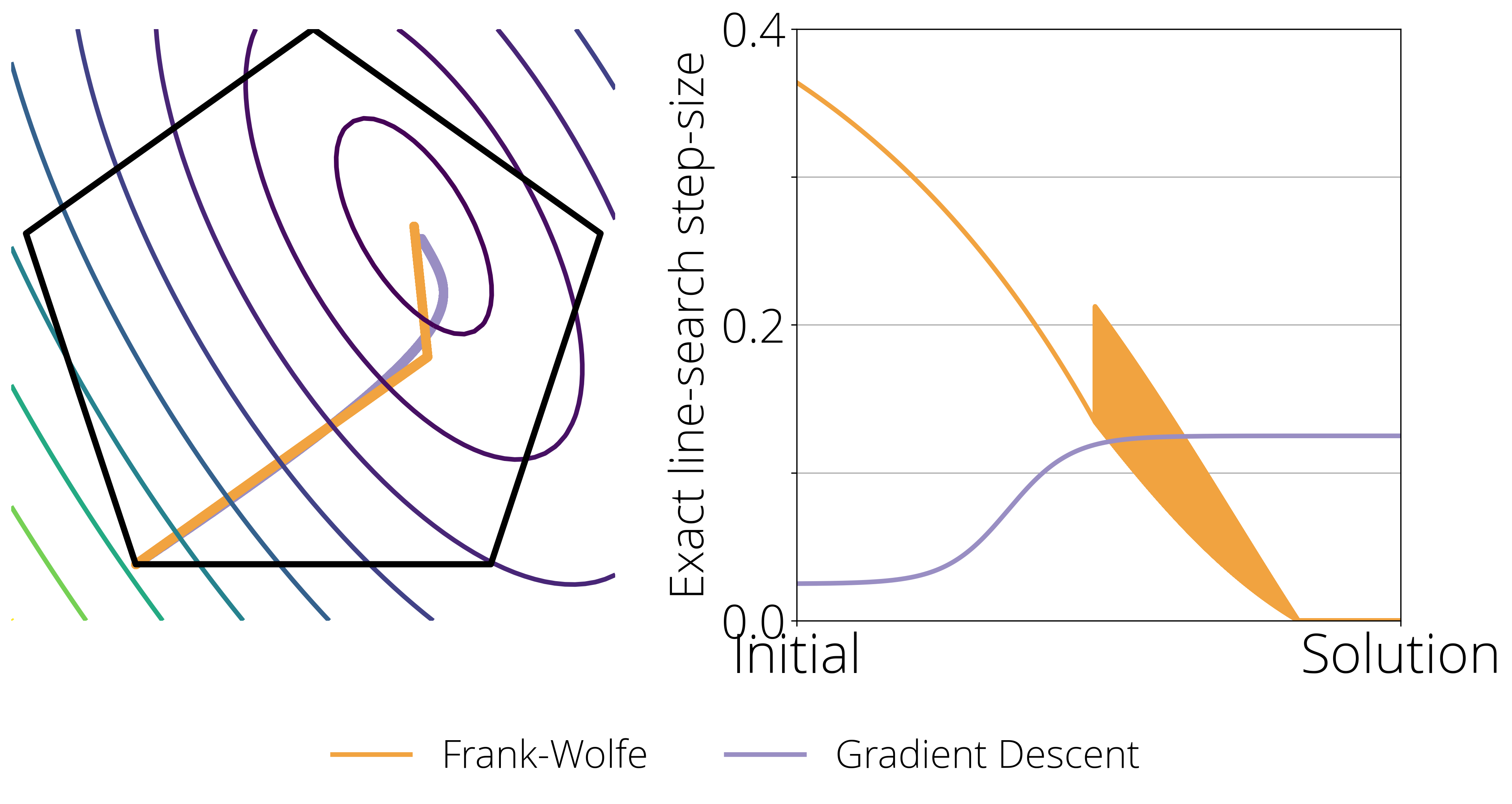
Think about the next determine. Within the left hand facet we present a toy 2-dimensional constrained drawback, the place the extent curves characterize the worth of the target perform, the pentagon are the constrain set, and the orange and violet curve reveals the trail taken by Frank-Wolfe and Gradient descent respectively when the step-size goes to zero (left). The suitable facet plot reveals the optimum step-size (decided by actual line-search) at each level of the optimization path.
This final plot highlights two essential variations between the Frank-Wolfe and Gradient Descent that we want to bear in mind when designing a step-size scheduler:

![]()
- Stability and convergence to zero. Gradient Descent converges with a relentless (non-zero) step-size, Frank-Wolfe does not. It requires a lowering step-size to anneal the (probably non-zero) magnitude of the replace.
- Zig-zagging. When near the optimum, the Frank-Wolfe algorithm usually reveals a zig-zagging habits, the place the chosen vertex $d_t$ within the replace oscillates between two vertices. The most effective step-size is perhaps completely different in these two instructions, and so a superb technique ought to have the ability to shortly alternate between two completely different step-sizes.
Dissecting the Demyanov-Rubinov step-size
Understanding the Demyanov-Rubinov step-size shall be essential to creating an efficient adaptive step-size within the subsequent part.
The Demyanov-Rubinov step-size may be derived from a quadratic higher sure on the target.
It is a classical end in optimization {that a} perform with $Lipschitz$-Lipschitz gradient admits the next quadratic higher sure for some fixed $Lipschitz$ and all $xx, yy$ within the area:
f(yy) leq f(xx) + langle nabla f(xx), yy – xx rangle + frac{Lipschitz}{2}|xx – yy|^2~.
finish{equation}
Making use of this inequality on the present and subsequent FW iterate $(xx = xx_t, yy = xx_{t} + stepsize dd_t)$ we get hold of
start{equation}label{eq:l_smooth2}
f(xx_t + stepsize dd_t) leq f(xx_t) – stepsize g_t + frac{stepsize^2 Lipschitz}{2}|dd_t|^2~.
finish{equation}
The suitable hand facet is a quadratic perform of $stepsize$. Minimizing it topic to the constraint $stepsize in [0, 1]$ –to ensure the iterates stay the area – offers the next resolution:
stepsize_t^textual content{DR} = minleft{ frac{g_t}dd_t, 1right},,
finish{equation}
which is the DR step-size from Eq. eqref{eq:ls_demyanov}.
Frank-Wolfe with backtracking line-search
The primary downside of the DR step-size is that it requires information of the Lipschitz fixed. This limits its usefulness as a result of, first, it is perhaps pricey to compute this fixed, and secondly, this fixed is a international higher sure on the curvature, resulting in suboptimal step-sizes in areas the place the native curvature is perhaps a lot smaller.
However there is a manner round this limitation. It is potential estimate a step-size such that it ensures a sure lower of the target with out utilizing international constants. The primary work to try this was (Dunn 1980)
On this algorithm, as an alternative of counting on the quadratic higher sure given by the Lipschitz fixed, we assemble an area quadratic approximation at $xx_t$. This quadratic perform is analogous to eqref{eq:l_smooth2}, however the place the worldwide Lipschitz fixed is changed by the possibly a lot smaller native fixed $LocalLipschitz_t$:
start{equation}
Q_t(stepsize, LocalLipschitz_t) defas f(xx_t) – stepsize g_t + frac{stepsize^2 LocalLipschitz_t}{2} |dd_t|^2,.
finish{equation}
As with the Demyanov-Rubinov step-size, we are going to select the step-size that minimizes the approximation on the $[0, 1]$ interval, that’s
start{equation}
stepsize_{t} = minleft{ frac{g_t}dd_t, 1right},.
finish{equation}
Be aware that this step-size has a really related type because the DR step-size, however with $LocalLipschitz_t$ changing $Lipschitz$.
That is all fantastic and good, thus far it appears we have solely displaced the issue from estimating $Lipschitz$ to estimating $LocalLipschitz_t$.
Right here is the place issues flip attention-grabbing: there is a method to estimate $LocalLipschitz_t$, that’s each handy and likewise offers robust theoretical ensures.
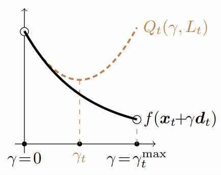
The adequate lower situation ensures that the quadratic approximation is an higher sure at its constrained minimal of the line-search goal.
For this, we’ll select the $LocalLipschitz_t$ that makes the quadratic approximation an higher sure on the subsequent iterate:
start{equation}label{eq:sufficient_decrease}
f(xx_{t+1}) leq Q_t(stepsize_t, LocalLipschitz_t) ,.
finish{equation}
This fashion, we will assure that the backtracking line-search step-size makes a minimum of as a lot progress as actual line-search within the quadratic approximation.
There are a lot of values of $LocalLipschitz_t$ that confirm this situation. For instance, from the $Lipschitz$-smooth inequality eqref{eq:l_smooth2} we all know that any $LocalLipschitz_t geq Lipschitz$ shall be a legitimate selection. Nonetheless, values of $LocalLipschitz_t$ which are a lot smaller than $Lipschitz$ would be the most attention-grabbing, as these will result in bigger step-sizes.
In observe there’s little worth in spending an excessive amount of time discovering the smallest potential worth of $LocalLipschitz_t$, and the most typical technique consists in initializing this worth a bit smaller than the one used within the earlier iterate (for instance $0.99 occasions LocalLipschitz_{t-1}$), and proper if vital.
Under is the complete Frank-Wolfe algorithm with backtracking line-search. The elements answerable for the estimation of the step-size are between the feedback /* start of backtracking line-search */ and /* finish of backtracking line-search */ .
Frank-Wolfe with backtracking line-search
Enter: preliminary guess $xx_0$, tolerance $delta > 0$, backtracking line-search parameters $tau > 1$, $eta leq 1$, preliminary guess for $LocalLipschitz_{-1}$.
$quadboldsymbol{s}_t in argmax_{boldsymbol{s} in mathcal{D}} langle -nabla f(boldsymbol{x}_t), boldsymbol{s}rangle$
Set $dd_t = ss_t – xx_t$ and $g_t = langle – nabla f(xx_t), dd_trangle$
/* start of backtracking line-search */
$LocalLipschitz_t = eta LocalLipschitz_{t-1}$
$stepsize_t = minleft{{{g}_t}/{(LocalLipschitz_t|dd_t|^{2})}, 1right}$
Whereas $f(xx_t + stepsize_t dd_t) > Q_t(stepsize_t, LocalLipschitz_t) $ do
/* finish of backtracking line-search */
$boldsymbol{x}_{t+1} = boldsymbol{x}_t + {stepsize}_t dd_t~.$
$textbf{finish For loop}$
$textbf{return } xx_t$
Let’s unpack what occurs contained in the backtracking line-search block. The block begins by selecting a relentless that could be a issue of $eta$ smaller than the one given by the earlier iterate. If $eta = 1$, then it is going to be precisely the identical than the earlier iterate, but when $eta$ is smaller than $1$ (I discovered $eta = 0.9$ to be an affordable default), this can end in a candidate worth of $LocalLipschitz_t$ that’s smaller than the one used within the earlier iterate. That is finished to make sure this fixed can lower if we transfer to a area with smaller curvature.
Within the subsequent line the algorithm units a tentative worth for the step-size based mostly on the components REF utilizing the present (tentative) worth for $LocalLipschitz_t$. The subsequent line is a Whereas loop that will increase $LocalLipschitz_t$ till it verifies the adequate lower situation eqref{eq:sufficient_decrease}
The algorithm will not be totally agnostic to the native
Lipschitz fixed, because it nonetheless requires to set an preliminary worth for this fixed, $LocalLipschitz_{-1}$. One heuristic that I discovered works properly in observe is to initialize it to the (approximate) native curvature alongside the replace route. For this, choose a small $varepsilon$, say $varepsilon = 10^{-3}$ and set
start{equation}
LocalLipschitz_{-1} = fracnabla f(xx_0) – nabla f(xx_0 + varepsilon dd_0),.
finish{equation}
Convergence charges
By the adequate lower situation we’ve got at every iteration
start{align}
mathcal{P}(xx_{t+1}) &leq mathcal{P}(xx_t) – stepsize_t g_t +
frac{stepsize_t^2 LocalLipschitz_t}{2}|ss_t – xx_t|^2
&leq mathcal{P}(xx_t) – xi_t g_t +
frac{xi_t^2 LocalLipschitz_t}{2}|ss_t – xx_t|^2 textual content{ for any $xi_t in [0, 1]$}
&leq mathcal{P}(xx_t) – xi_t g_t +
frac{xi_t^2 tau Lipschitz}{2}|ss_t – xx_t|^2 textual content{ for any $xi_t in [0, 1]$},,
finish{align}
the place within the second inequality we’ve got used the truth that $stepsize_t$ is the minimizer of this right-hand facet over the $[0, 1]$ interval, and so it is an higher sure on any worth on this interval. Within the third inequality we’ve got used that the adequate lower situation is verified for any $LocalLipschitz geq Lipschitz$, and so the backtracking loop can not convey its worth under $tau LocalLipschitz$, so long as it was initialized with a price above this fixed.
The final identification is similar one we used as start line in Theorem 3 of the second a part of these notes to point out the sublinear convergence for convex goals (with a $Lipschitz$ as an alternative of $tau Lipschitz$). Following the identical proof then yields a $mathcal{O}(frac{1}{t})$ convergence fee on the primal-dual hole, with $Lipschitz$ changed by $tau Lipschitz$.
Our paper
Benchmarks
The empirical speedup of the backtracking line-search is large, typically as much as an order of magnitude. Under I examine Frank-Wolfe with backtracking line-search (denoted adaptive
) and with Demyanov-Rubinov step-size (denoted Lipschitz
). All the issues are cases of logistic regression with $ell_1$ regularization on completely different datasets utilizing the copt software program bundle.
adaptive) and Demyanov-Rubinov (denoted
Lipschitz) on completely different datasets.
Citing
For those who’ve discovered this weblog publish helpful, please take into account citing it is full-length companion paper. This paper extends the speculation introduced right here to different Frank-Wolfe variants equivalent to Away-steps Frank-Wolfe and Pairwise Frank-Wolfe. Moreover, it reveals that these variants preserve its linear convergence with backtracking line-search.
Linearly Convergent Frank-Wolfe with Backtracking Line-Search, Fabian Pedregosa, Geoffrey Negiar, Armin Askari, Martin Jaggi. Proceedings of the twenty second Worldwide Convention on Synthetic Intelligence and Statistics (AISTATS), 2020
Bibtex entry:
  @inproceedings{pedregosa2020linearly,
    title={Linearly Convergent Frank-Wolfe with Backtracking Line-Search},
    creator={Pedregosa, Fabian and Negiar, Geoffrey and Askari, Armin and Jaggi, Martin},
    booktitle={Worldwide Convention on Synthetic Intelligence and Statistics},
    sequence = {Proceedings of Machine Studying Analysis},
    yr={2020}
  }
Thanks
Thanks Geoffrey Negiar and Quentin Berthet for suggestions on this publish.