Friday, April 19, 2024
HomeMatlabClimate Forecasting in MATLAB for the WiDS Datathon 2023

Climate Forecasting in MATLAB for the WiDS Datathon 2023


In immediately’s weblog, Grace Woolson will likely be displaying how individuals of the Ladies in Knowledge Science (WiDS) Datathon 2023 and others can get began utilizing MATLAB for climate forecasting utilizing machine studying!

Introduction

Hiya! In the present day, I’m going to indicate an instance of how you should utilize MATLAB for the WiDS Datathon 2023. This yr’s problem duties individuals with making a mannequin that may predict long-term temperature forecasts, which will help communities adapt to excessive climate occasions usually attributable to local weather change. WiDS individuals will submit their forecasts on Kaggle. This tutorial will stroll via the next steps of the model-making course of:
  1. Importing a Tabular Dataset
  2. Preprocessing Knowledge
  3. Coaching and Evaluating a Machine Studying Mannequin
  4. Making New Predictions and Exporting Predictions
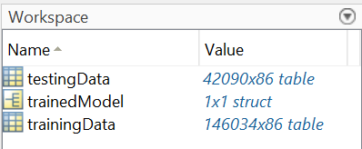
MathWorks is pleased to help individuals of the Ladies in Knowledge Science Datathon 2023 by offering complimentary MATLAB licenses, tutorials, workshops, and extra assets. To request complimentary licenses for you and your teammates, go to this MathWorks website, click on the “Request Software program” button, and fill out the software program request type.
To register for the competitors and entry the dataset, go to the Kaggle web page, sign-in or register for an account, and click on the ‘Be part of Competitors’ button. By accepting the foundations for the competitors, it is possible for you to to obtain the problem datasets obtainable on the ‘Knowledge’ tab.

Import Knowledge

First, we have to carry the coaching information into the MATLAB workspace. For this tutorial, I will likely be utilizing a subset of the general problem dataset, so the recordsdata proven under will differ from those you might be offered. The datasets I will likely be utilizing are:
  • Coaching information (practice.xlsx)
  • Testing information (check.xlsx)
The info is in tabular type, so we will use the readtable perform to import the info.
trainingData = readtable(‘practice.xlsx’, ‘VariableNamingRule’, ‘protect’);
testingData = readtable(‘check.xlsx’, ‘VariableNamingRule’, ‘protect’);
For the reason that tables are so giant, we don’t wish to present the entire dataset without delay, as a result of it would take up the whole display! Let’s use the head perform to show the highest 8 rows of the tables, so we will get a way of what information we’re working with.
head(trainingData)
lat lon start_date cancm3_0_x cancm4_0_x ccsm3_0_x ccsm4_0_x cfsv2_0_x gfdl-flor-a_0_x gfdl-flor-b_0_x gfdl_0_x nasa_0_x nmme0_mean_x cancm3_x cancm4_x ccsm3_x ccsm4_x cfsv2_x gfdl_x gfdl-flor-a_x gfdl-flor-b_x nasa_x nmme_mean_x cancm3_y cancm4_y ccsm3_y ccsm4_y cfsv2_y gfdl_y gfdl-flor-a_y gfdl-flor-b_y nasa_y nmme_mean_y cancm3_0_y cancm4_0_y ccsm3_0_y ccsm4_0_y cfsv2_0_y gfdl-flor-a_0_y gfdl-flor-b_0_y gfdl_0_y nasa_0_y nmme0_mean_y cancm3_0_x_1 cancm4_0_x_1 ccsm3_0_x_1 ccsm4_0_x_1 cfsv2_0_x_1 gfdl-flor-a_0_x_1 gfdl-flor-b_0_x_1 gfdl_0_x_1 nasa_0_x_1 nmme0_mean_x_1 tmp2m cancm3_x_1 cancm4_x_1 ccsm3_x_1 ccsm4_x_1 cfsv2_x_1 gfdl_x_1 gfdl-flor-a_x_1 gfdl-flor-b_x_1 nasa_x_1 nmme_mean_x_1 cancm3_y_1 cancm4_y_1 ccsm3_y_1 ccsm4_y_1 cfsv2_y_1 gfdl_y_1 gfdl-flor-a_y_1 gfdl-flor-b_y_1 nasa_y_1 nmme_mean_y_1 cancm3_0_y_1 cancm4_0_y_1 ccsm3_0_y_1 ccsm4_0_y_1 cfsv2_0_y_1 gfdl-flor-a_0_y_1 gfdl-flor-b_0_y_1 gfdl_0_y_1 nasa_0_y_1 nmme0_mean_y_1
___ ___ ___________ __________ __________ _________ _________ _________ _______________ _______________ ________ ________ ____________ ________ ________ _______ _______ _______ ______ _____________ _____________ ______ ___________ ________ ________ _______ _______ _______ ______ _____________ _____________ ______ ___________ __________ __________ _________ _________ _________ _______________ _______________ ________ ________ ____________ ____________ ____________ ___________ ___________ ___________ _________________ _________________ __________ __________ ______________ ______ __________ __________ _________ _________ _________ ________ _______________ _______________ ________ _____________ __________ __________ _________ _________ _________ ________ _______________ _______________ ________ _____________ ____________ ____________ ___________ ___________ ___________ _________________ _________________ __________ __________ ______________27 261 01-Jan-2016 10.801 12.686 11.962 13.5 13.012 11.99 12.29 8.5611 13.64 12.049 9.8245 11.061 10.498 10.408 11.857 8.3761 11.315 11.775 12.281 10.822 13.191 16.105 30.301 26.116 43.048 40.007 26.308 24.571 26.924 27.397 35.156 28.155 30.717 34.552 28.183 28.298 28.652 34.429 37.595 31.748 25.938 16.519 23.387 21.876 39.836 21.261 14.133 36.942 29.398 25.477 12.044 29.098 21.265 42.821 28.231 40.159 62.355 24.896 24.933 22.981 32.971 9.2216 12.444 10.616 10.461 11.401 7.7597 12.194 11.664 12.213 10.886 16.57 18.283 15.485 18.897 17.87 16.714 17.432 13.391 20.003 17.183
27 261 02-Jan-2016 10.801 12.686 11.962 13.5 13.012 11.99 12.29 8.5611 13.64 12.049 9.8245 11.061 10.498 10.408 11.857 8.3761 11.315 11.775 12.281 10.822 13.191 16.105 30.301 26.116 43.048 40.007 26.308 24.571 26.924 27.397 35.156 28.155 30.717 34.552 28.183 28.298 28.652 34.429 37.595 31.748 25.938 16.519 23.387 21.876 39.836 21.261 14.133 36.942 29.398 25.477 12.631 29.098 21.265 42.821 28.231 40.159 62.355 24.896 24.933 22.981 32.971 9.2216 12.444 10.616 10.461 11.401 7.7597 12.194 11.664 12.213 10.886 16.57 18.283 15.485 18.897 17.87 16.714 17.432 13.391 20.003 17.183
27 261 03-Jan-2016 10.801 12.686 11.962 13.5 13.012 11.99 12.29 8.5611 13.64 12.049 9.8245 11.061 10.498 10.408 11.857 8.3761 11.315 11.775 12.281 10.822 13.191 16.105 30.301 26.116 43.048 40.007 26.308 24.571 26.924 27.397 35.156 28.155 30.717 34.552 28.183 28.298 28.652 34.429 37.595 31.748 25.938 16.519 23.387 21.876 39.836 21.261 14.133 36.942 29.398 25.477 13.305 29.098 21.265 42.821 28.231 40.159 62.355 24.896 24.933 22.981 32.971 9.2216 12.444 10.616 10.461 11.401 7.7597 12.194 11.664 12.213 10.886 16.57 18.283 15.485 18.897 17.87 16.714 17.432 13.391 20.003 17.183
27 261 04-Jan-2016 10.801 12.686 11.962 13.5 13.012 11.99 12.29 8.5611 13.64 12.049 9.8245 11.061 10.498 10.408 11.857 8.3761 11.315 11.775 12.281 10.822 13.191 16.105 30.301 26.116 43.048 40.007 26.308 24.571 26.924 27.397 35.156 28.155 30.717 34.552 28.183 28.298 28.652 34.429 37.595 31.748 25.938 16.519 23.387 21.876 39.836 21.261 14.133 36.942 29.398 25.477 13.396 29.098 21.265 42.821 28.231 40.159 62.355 24.896 24.933 22.981 32.971 9.2216 12.444 10.616 10.461 11.401 7.7597 12.194 11.664 12.213 10.886 16.57 18.283 15.485 18.897 17.87 16.714 17.432 13.391 20.003 17.183
27 261 05-Jan-2016 10.801 12.686 11.962 13.5 13.012 11.99 12.29 8.5611 13.64 12.049 9.8245 11.061 10.498 10.408 11.857 8.3761 11.315 11.775 12.281 10.822 13.191 16.105 30.301 26.116 43.048 40.007 26.308 24.571 26.924 27.397 35.156 28.155 30.717 34.552 28.183 28.298 28.652 34.429 37.595 31.748 25.938 16.519 23.387 21.876 39.836 21.261 14.133 36.942 29.398 25.477 13.627 29.098 21.265 42.821 28.231 40.159 62.355 24.896 24.933 22.981 32.971 9.2216 12.444 10.616 10.461 11.401 7.7597 12.194 11.664 12.213 10.886 16.57 18.283 15.485 18.897 17.87 16.714 17.432 13.391 20.003 17.183
27 261 06-Jan-2016 10.801 12.686 11.962 13.5 13.012 11.99 12.29 8.5611 13.64 12.049 9.2216 12.444 10.616 10.461 11.401 7.7597 12.194 11.664 12.213 10.886 13.191 16.105 30.301 26.116 43.048 40.007 26.308 24.571 26.924 27.397 25.938 16.519 23.387 21.876 39.836 21.261 14.133 36.942 29.398 25.477 25.938 16.519 23.387 21.876 39.836 21.261 14.133 36.942 29.398 25.477 13.999 13.191 16.105 30.301 26.116 43.048 40.007 26.308 24.571 26.924 27.397 9.2216 12.444 10.616 10.461 11.401 7.7597 12.194 11.664 12.213 10.886 10.801 12.686 11.962 13.5 13.012 11.99 12.29 8.5611 13.64 12.049
27 261 07-Jan-2016 10.801 12.686 11.962 13.5 13.012 11.99 12.29 8.5611 13.64 12.049 9.2216 12.444 10.616 10.461 11.401 7.7597 12.194 11.664 12.213 10.886 13.191 16.105 30.301 26.116 43.048 40.007 26.308 24.571 26.924 27.397 25.938 16.519 23.387 21.876 39.836 21.261 14.133 36.942 29.398 25.477 25.938 16.519 23.387 21.876 39.836 21.261 14.133 36.942 29.398 25.477 14.223 13.191 16.105 30.301 26.116 43.048 40.007 26.308 24.571 26.924 27.397 9.2216 12.444 10.616 10.461 11.401 7.7597 12.194 11.664 12.213 10.886 10.801 12.686 11.962 13.5 13.012 11.99 12.29 8.5611 13.64 12.049
27 261 08-Jan-2016 10.801 12.686 11.962 13.5 13.012 11.99 12.29 8.5611 13.64 12.049 9.2216 12.444 10.616 10.461 11.401 7.7597 12.194 11.664 12.213 10.886 13.191 16.105 30.301 26.116 43.048 40.007 26.308 24.571 26.924 27.397 25.938 16.519 23.387 21.876 39.836 21.261 14.133 36.942 29.398 25.477 25.938 16.519 23.387 21.876 39.836 21.261 14.133 36.942 29.398 25.477 14.248 13.191 16.105 30.301 26.116 43.048 40.007 26.308 24.571 26.924 27.397 9.2216 12.444 10.616 10.461 11.401 7.7597 12.194 11.664 12.213 10.886 10.801 12.686 11.962 13.5 13.012 11.99 12.29 8.5611 13.64 12.049
head(testingData)
lat lon start_date cancm3_0_x cancm4_0_x ccsm3_0_x ccsm4_0_x cfsv2_0_x gfdl-flor-a_0_x gfdl-flor-b_0_x gfdl_0_x nasa_0_x nmme0_mean_x cancm3_x cancm4_x ccsm3_x ccsm4_x cfsv2_x gfdl_x gfdl-flor-a_x gfdl-flor-b_x nasa_x nmme_mean_x cancm3_y cancm4_y ccsm3_y ccsm4_y cfsv2_y gfdl_y gfdl-flor-a_y gfdl-flor-b_y nasa_y nmme_mean_y cancm3_0_y cancm4_0_y ccsm3_0_y ccsm4_0_y cfsv2_0_y gfdl-flor-a_0_y gfdl-flor-b_0_y gfdl_0_y nasa_0_y nmme0_mean_y cancm3_0_x_1 cancm4_0_x_1 ccsm3_0_x_1 ccsm4_0_x_1 cfsv2_0_x_1 gfdl-flor-a_0_x_1 gfdl-flor-b_0_x_1 gfdl_0_x_1 nasa_0_x_1 nmme0_mean_x_1 tmp2m cancm3_x_1 cancm4_x_1 ccsm3_x_1 ccsm4_x_1 cfsv2_x_1 gfdl_x_1 gfdl-flor-a_x_1 gfdl-flor-b_x_1 nasa_x_1 nmme_mean_x_1 cancm3_y_1 cancm4_y_1 ccsm3_y_1 ccsm4_y_1 cfsv2_y_1 gfdl_y_1 gfdl-flor-a_y_1 gfdl-flor-b_y_1 nasa_y_1 nmme_mean_y_1 cancm3_0_y_1 cancm4_0_y_1 ccsm3_0_y_1 ccsm4_0_y_1 cfsv2_0_y_1 gfdl-flor-a_0_y_1 gfdl-flor-b_0_y_1 gfdl_0_y_1 nasa_0_y_1 nmme0_mean_y_1
___ ___ ___________ __________ __________ _________ _________ _________ _______________ _______________ ________ ________ ____________ ________ ________ _______ _______ _______ ______ _____________ _____________ ______ ___________ ________ ________ _______ _______ _______ ______ _____________ _____________ ______ ___________ __________ __________ _________ _________ _________ _______________ _______________ ________ ________ ____________ ____________ ____________ ___________ ___________ ___________ _________________ _________________ __________ __________ ______________ ______ __________ __________ _________ _________ _________ ________ _______________ _______________ ________ _____________ __________ __________ _________ _________ _________ ________ _______________ _______________ ________ _____________ ____________ ____________ ___________ ___________ ___________ _________________ _________________ __________ __________ ______________38 238 01-Jan-2016 7.3796 8.3793 8.5218 9.3342 9.508 10.423 10.946 9.3034 9.376 9.2413 6.4785 7.2476 8.747 10.039 9.444 7.7948 10.142 10.421 8.4113 8.7472 67.619 63.328 78.491 71.75 98.552 61.833 71.848 66.141 54.315 70.431 23.973 23.875 26.89 14.057 36.966 34.703 30.382 35.169 31.349 28.596 60.347 30.144 66.325 43.001 79.737 48.759 57.888 69.24 45.733 55.686 9.0021 71.945 84.607 56.394 80.506 123.53 57.872 92.886 107.55 69.046 82.703 7.0177 8.0908 8.0417 9.4876 8.3799 8.738 10.34 10.312 8.6557 8.7848 8.9173 9.2217 10.978 12.627 11.894 13.353 12.966 12.68 13.138 11.753
38 238 02-Jan-2016 7.3796 8.3793 8.5218 9.3342 9.508 10.423 10.946 9.3034 9.376 9.2413 6.4785 7.2476 8.747 10.039 9.444 7.7948 10.142 10.421 8.4113 8.7472 67.619 63.328 78.491 71.75 98.552 61.833 71.848 66.141 54.315 70.431 23.973 23.875 26.89 14.057 36.966 34.703 30.382 35.169 31.349 28.596 60.347 30.144 66.325 43.001 79.737 48.759 57.888 69.24 45.733 55.686 9.4104 71.945 84.607 56.394 80.506 123.53 57.872 92.886 107.55 69.046 82.703 7.0177 8.0908 8.0417 9.4876 8.3799 8.738 10.34 10.312 8.6557 8.7848 8.9173 9.2217 10.978 12.627 11.894 13.353 12.966 12.68 13.138 11.753
38 238 03-Jan-2016 7.3796 8.3793 8.5218 9.3342 9.508 10.423 10.946 9.3034 9.376 9.2413 6.4785 7.2476 8.747 10.039 9.444 7.7948 10.142 10.421 8.4113 8.7472 67.619 63.328 78.491 71.75 98.552 61.833 71.848 66.141 54.315 70.431 23.973 23.875 26.89 14.057 36.966 34.703 30.382 35.169 31.349 28.596 60.347 30.144 66.325 43.001 79.737 48.759 57.888 69.24 45.733 55.686 9.7816 71.945 84.607 56.394 80.506 123.53 57.872 92.886 107.55 69.046 82.703 7.0177 8.0908 8.0417 9.4876 8.3799 8.738 10.34 10.312 8.6557 8.7848 8.9173 9.2217 10.978 12.627 11.894 13.353 12.966 12.68 13.138 11.753
38 238 04-Jan-2016 7.3796 8.3793 8.5218 9.3342 9.508 10.423 10.946 9.3034 9.376 9.2413 6.4785 7.2476 8.747 10.039 9.444 7.7948 10.142 10.421 8.4113 8.7472 67.619 63.328 78.491 71.75 98.552 61.833 71.848 66.141 54.315 70.431 23.973 23.875 26.89 14.057 36.966 34.703 30.382 35.169 31.349 28.596 60.347 30.144 66.325 43.001 79.737 48.759 57.888 69.24 45.733 55.686 10.066 71.945 84.607 56.394 80.506 123.53 57.872 92.886 107.55 69.046 82.703 7.0177 8.0908 8.0417 9.4876 8.3799 8.738 10.34 10.312 8.6557 8.7848 8.9173 9.2217 10.978 12.627 11.894 13.353 12.966 12.68 13.138 11.753
38 238 05-Jan-2016 7.3796 8.3793 8.5218 9.3342 9.508 10.423 10.946 9.3034 9.376 9.2413 6.4785 7.2476 8.747 10.039 9.444 7.7948 10.142 10.421 8.4113 8.7472 67.619 63.328 78.491 71.75 98.552 61.833 71.848 66.141 54.315 70.431 23.973 23.875 26.89 14.057 36.966 34.703 30.382 35.169 31.349 28.596 60.347 30.144 66.325 43.001 79.737 48.759 57.888 69.24 45.733 55.686 10.35 71.945 84.607 56.394 80.506 123.53 57.872 92.886 107.55 69.046 82.703 7.0177 8.0908 8.0417 9.4876 8.3799 8.738 10.34 10.312 8.6557 8.7848 8.9173 9.2217 10.978 12.627 11.894 13.353 12.966 12.68 13.138 11.753
38 238 06-Jan-2016 7.3796 8.3793 8.5218 9.3342 9.508 10.423 10.946 9.3034 9.376 9.2413 7.0177 8.0908 8.0417 9.4876 8.3799 8.738 10.34 10.312 8.6557 8.7848 67.619 63.328 78.491 71.75 98.552 61.833 71.848 66.141 54.315 70.431 60.347 30.144 66.325 43.001 79.737 48.759 57.888 69.24 45.733 55.686 60.347 30.144 66.325 43.001 79.737 48.759 57.888 69.24 45.733 55.686 10.59 67.619 63.328 78.491 71.75 98.552 61.833 71.848 66.141 54.315 70.431 7.0177 8.0908 8.0417 9.4876 8.3799 8.738 10.34 10.312 8.6557 8.7848 7.3796 8.3793 8.5218 9.3342 9.508 10.423 10.946 9.3034 9.376 9.2413
38 238 07-Jan-2016 7.3796 8.3793 8.5218 9.3342 9.508 10.423 10.946 9.3034 9.376 9.2413 7.0177 8.0908 8.0417 9.4876 8.3799 8.738 10.34 10.312 8.6557 8.7848 67.619 63.328 78.491 71.75 98.552 61.833 71.848 66.141 54.315 70.431 60.347 30.144 66.325 43.001 79.737 48.759 57.888 69.24 45.733 55.686 60.347 30.144 66.325 43.001 79.737 48.759 57.888 69.24 45.733 55.686 10.674 67.619 63.328 78.491 71.75 98.552 61.833 71.848 66.141 54.315 70.431 7.0177 8.0908 8.0417 9.4876 8.3799 8.738 10.34 10.312 8.6557 8.7848 7.3796 8.3793 8.5218 9.3342 9.508 10.423 10.946 9.3034 9.376 9.2413
38 238 08-Jan-2016 7.3796 8.3793 8.5218 9.3342 9.508 10.423 10.946 9.3034 9.376 9.2413 7.0177 8.0908 8.0417 9.4876 8.3799 8.738 10.34 10.312 8.6557 8.7848 67.619 63.328 78.491 71.75 98.552 61.833 71.848 66.141 54.315 70.431 60.347 30.144 66.325 43.001 79.737 48.759 57.888 69.24 45.733 55.686 60.347 30.144 66.325 43.001 79.737 48.759 57.888 69.24 45.733 55.686 10.995 67.619 63.328 78.491 71.75 98.552 61.833 71.848 66.141 54.315 70.431 7.0177 8.0908 8.0417 9.4876 8.3799 8.738 10.34 10.312 8.6557 8.7848 7.3796 8.3793 8.5218 9.3342 9.508 10.423 10.946 9.3034 9.376 9.2413
Now we will see the names of all the columns (also referred to as variables) and get a way of their datatypes, which can make it a lot simpler to work with these tables. Discover that each datasets have the identical variable names. In case you look via all the variable names, you’ll see one known as ‘tmp2m’ – that is the column we will likely be coaching a mannequin to foretell, additionally known as the response variable.
You will need to have a coaching and testing set with identified outputs, so you’ll be able to see how properly your mannequin performs on unseen information. On this case, it’s cut up forward of time, however you could want to separate your coaching set manually. For instance, you probably have one dataset in a 100,000-row desk known as ‘train_data’, the instance code under would randomly cut up this desk into 80% coaching and 20% testing information. These percentages are comparatively normal when distributing coaching and testing information, however you could wish to check out totally different values when making your datasets!
[trainInd, ~, testInd] = dividerand(100000, .8, 0, .2);
trainingData = train_data(trainInd, :);
testingData = train_data(testInd, :);

Preprocess Knowledge

Now that the info is within the workspace, we have to take some steps to wash and format it so it may be used to coach a machine studying mannequin. We will use the abstract perform to see the datatype and statistical details about every variable:
abstract(trainingData)

Variables:

lat: 146034×1 double

Values:

Min 27
Median 42
Max 49

lon: 146034×1 double

Values:

Min 236
Median 252
Max 266

start_date: 146034×1 datetime

Values:

Min 01-Jan-2016 00:00:00
Median 01-Jul-2016 12:00:00
Max 31-Dec-2016 00:00:00

cancm3_0_x: 146034×1 double

Values:

Min -12.902
Median 10.535
Max 36.077

cancm4_0_x: 146034×1 double

Values:

Min -13.276
Median 12.512
Max 35.795

ccsm3_0_x: 146034×1 double

Values:

Min -11.75
Median 10.477
Max 32.974

ccsm4_0_x: 146034×1 double

Values:

Min -13.264
Median 12.315
Max 34.311

cfsv2_0_x: 146034×1 double

Values:

Min -11.175
Median 11.34
Max 35.749

gfdl-flor-a_0_x: 146034×1 double

Values:

Min -12.85
Median 11.831
Max 37.416

gfdl-flor-b_0_x: 146034×1 double

Values:

Min -13.52
Median 11.837
Max 37.34

gfdl_0_x: 146034×1 double

Values:

Min -11.165
Median 10.771
Max 36.117

nasa_0_x: 146034×1 double

Values:

Min -19.526
Median 14.021
Max 38.22

nmme0_mean_x: 146034×1 double

Values:

Min -12.194
Median 11.893
Max 34.879

cancm3_x: 146034×1 double

Values:

Min -12.969
Median 9.9291
Max 36.235

cancm4_x: 146034×1 double

Values:

Min -12.483
Median 12.194
Max 38.378

ccsm3_x: 146034×1 double

Values:

Min -13.033
Median 10.368
Max 33.42

ccsm4_x: 146034×1 double

Values:

Min -14.28
Median 12.254
Max 34.957

cfsv2_x: 146034×1 double

Values:

Min -14.683
Median 10.897
Max 35.795

gfdl_x: 146034×1 double

Values:

Min -9.8741
Median 10.476
Max 35.95

gfdl-flor-a_x: 146034×1 double

Values:

Min -13.021
Median 11.15
Max 37.834

gfdl-flor-b_x: 146034×1 double

Values:

Min -12.557
Median 11.117
Max 37.192

nasa_x: 146034×1 double

Values:

Min -21.764
Median 13.721
Max 38.154

nmme_mean_x: 146034×1 double

Values:

Min -13.042
Median 11.354
Max 35.169

cancm3_y: 146034×1 double

Values:

Min 0.075757
Median 18.56
Max 124.58

cancm4_y: 146034×1 double

Values:

Min 0.02538
Median 16.296
Max 137.78

ccsm3_y: 146034×1 double

Values:

Min 4.5927e-05
Median 24.278
Max 126.36

ccsm4_y: 146034×1 double

Values:

Min 0.096667
Median 24.455
Max 204.37

cfsv2_y: 146034×1 double

Values:

Min 0.074655
Median 25.91
Max 156.7

gfdl_y: 146034×1 double

Values:

Min 0.0046441
Median 20.49
Max 133.88

gfdl-flor-a_y: 146034×1 double

Values:

Min 0.0044707
Median 20.438
Max 195.32

gfdl-flor-b_y: 146034×1 double

Values:

Min 0.0095625
Median 20.443
Max 187.15

nasa_y: 146034×1 double

Values:

Min 1.9478e-05
Median 17.98
Max 164.94

nmme_mean_y: 146034×1 double

Values:

Min 0.2073
Median 21.494
Max 132

cancm3_0_y: 146034×1 double

Values:

Min 0.016023
Median 19.365
Max 139.94

cancm4_0_y: 146034×1 double

Values:

Min 0.016112
Median 17.354
Max 160.04

ccsm3_0_y: 146034×1 double

Values:

Min 0.00043188
Median 21.729
Max 144.19

ccsm4_0_y: 146034×1 double

Values:

Min 0.02979
Median 23.642
Max 151.3

cfsv2_0_y: 146034×1 double

Values:

Min 0.01827
Median 25.095
Max 176.15

gfdl-flor-a_0_y: 146034×1 double

Values:

Min 0.0058198
Median 17.634
Max 184.7

gfdl-flor-b_0_y: 146034×1 double

Values:

Min 0.0045824
Median 16.937
Max 194.19

gfdl_0_y: 146034×1 double

Values:

Min 0.0030585
Median 19.379
Max 140.16

nasa_0_y: 146034×1 double

Values:

Min 0.00051379
Median 17.81
Max 167.31

nmme0_mean_y: 146034×1 double

Values:

Min 0.061258
Median 20.697
Max 140.1

cancm3_0_x_1: 146034×1 double

Values:

Min 0.016023
Median 19.436
Max 139.94

cancm4_0_x_1: 146034×1 double

Values:

Min 0.016112
Median 17.261
Max 160.04

ccsm3_0_x_1: 146034×1 double

Values:

Min 0.00043188
Median 21.75
Max 144.19

ccsm4_0_x_1: 146034×1 double

Values:

Min 0.02979
Median 23.45
Max 231.72

cfsv2_0_x_1: 146034×1 double

Values:

Min 0.01827
Median 25.096
Max 176.15

gfdl-flor-a_0_x_1: 146034×1 double

Values:

Min 0.0058198
Median 17.617
Max 217.6

gfdl-flor-b_0_x_1: 146034×1 double

Values:

Min 0.0045824
Median 16.915
Max 195.06

gfdl_0_x_1: 146034×1 double

Values:

Min 0.0030585
Median 19.411
Max 140.16

nasa_0_x_1: 146034×1 double

Values:

Min 0.00051379
Median 17.733
Max 180.77

nmme0_mean_x_1: 146034×1 double

Values:

Min 0.061258
Median 20.67
Max 140.1

tmp2m: 146034×1 double

Values:

Min -21.031
Median 12.742
Max 37.239

cancm3_x_1: 146034×1 double

Values:

Min 0.075757
Median 18.649
Max 124.58

cancm4_x_1: 146034×1 double

Values:

Min 0.02538
Median 16.588
Max 116.86

ccsm3_x_1: 146034×1 double

Values:

Min 4.5927e-05
Median 25.242
Max 134.15

ccsm4_x_1: 146034×1 double

Values:

Min 0.21704
Median 24.674
Max 204.37

cfsv2_x_1: 146034×1 double

Values:

Min 0.028539
Median 26.282
Max 154.39

gfdl_x_1: 146034×1 double

Values:

Min 0.0046441
Median 21.028
Max 142.5

gfdl-flor-a_x_1: 146034×1 double

Values:

Min 0.0044707
Median 21.322
Max 187.57

gfdl-flor-b_x_1: 146034×1 double

Values:

Min 0.0095625
Median 21.444
Max 193.19

nasa_x_1: 146034×1 double

Values:

Min 1.9478e-05
Median 17.963
Max 183.71

nmme_mean_x_1: 146034×1 double

Values:

Min 0.24096
Median 21.881
Max 124.19

cancm3_y_1: 146034×1 double

Values:

Min -11.839
Median 10.067
Max 36.235

cancm4_y_1: 146034×1 double

Values:

Min -11.809
Median 12.179
Max 38.378

ccsm3_y_1: 146034×1 double

Values:

Min -11.662
Median 10.552
Max 33.171

ccsm4_y_1: 146034×1 double

Values:

Min -14.66
Median 12.254
Max 34.891

cfsv2_y_1: 146034×1 double

Values:

Min -14.519
Median 10.99
Max 35.795

gfdl_y_1: 146034×1 double

Values:

Min -10.906
Median 10.555
Max 35.95

gfdl-flor-a_y_1: 146034×1 double

Values:

Min -12.995
Median 11.24
Max 37.834

gfdl-flor-b_y_1: 146034×1 double

Values:

Min -12.899
Median 11.255
Max 37.192

nasa_y_1: 146034×1 double

Values:

Min -21.459
Median 13.768
Max 38.154

nmme_mean_y_1: 146034×1 double

Values:

Min -13.219
Median 11.462
Max 35.169

cancm3_0_y_1: 146034×1 double

Values:

Min -12.902
Median 10.475
Max 36.077

cancm4_0_y_1: 146034×1 double

Values:

Min -13.276
Median 12.385
Max 35.795

ccsm3_0_y_1: 146034×1 double

Values:

Min -9.4298
Median 10.452
Max 32.974

ccsm4_0_y_1: 146034×1 double

Values:

Min -12.54
Median 12.237
Max 34.311

cfsv2_0_y_1: 146034×1 double

Values:

Min -10.862
Median 11.315
Max 35.749

gfdl-flor-a_0_y_1: 146034×1 double

Values:

Min -12.85
Median 11.831
Max 37.416

gfdl-flor-b_0_y_1: 146034×1 double

Values:

Min -13.52
Median 11.842
Max 37.34

gfdl_0_y_1: 146034×1 double

Values:

Min -9.2018
Median 10.658
Max 36.117

nasa_0_y_1: 146034×1 double

Values:

Min -19.526
Median 14.002
Max 38.22

nmme0_mean_y_1: 146034×1 double

Values:

Min -12.194
Median 11.861
Max 34.879

This exhibits that every one variables are doubles aside from the ‘start_time’ variable, which is a datetime, and isn’t appropriate with many machine studying algorithms. Let’s break this up into three separate predictors that could be extra useful when coaching our algorithms:
trainingData.Day = trainingData.start_date.Day;
trainingData.Month = trainingData.start_date.Month;
trainingData.12 months = trainingData.start_date.12 months;
trainingData.start_date = [];
I’m additionally going to maneuver the ‘tmp2m’ variable to the top, which can make it simpler to differentiate that that is the variable we wish to predict.
trainingData = movevars(trainingData, “tmp2m”, “After”, “12 months”);
head(trainingData)
lat lon cancm3_0_x cancm4_0_x ccsm3_0_x ccsm4_0_x cfsv2_0_x gfdl-flor-a_0_x gfdl-flor-b_0_x gfdl_0_x nasa_0_x nmme0_mean_x cancm3_x cancm4_x ccsm3_x ccsm4_x cfsv2_x gfdl_x gfdl-flor-a_x gfdl-flor-b_x nasa_x nmme_mean_x cancm3_y cancm4_y ccsm3_y ccsm4_y cfsv2_y gfdl_y gfdl-flor-a_y gfdl-flor-b_y nasa_y nmme_mean_y cancm3_0_y cancm4_0_y ccsm3_0_y ccsm4_0_y cfsv2_0_y gfdl-flor-a_0_y gfdl-flor-b_0_y gfdl_0_y nasa_0_y nmme0_mean_y cancm3_0_x_1 cancm4_0_x_1 ccsm3_0_x_1 ccsm4_0_x_1 cfsv2_0_x_1 gfdl-flor-a_0_x_1 gfdl-flor-b_0_x_1 gfdl_0_x_1 nasa_0_x_1 nmme0_mean_x_1 cancm3_x_1 cancm4_x_1 ccsm3_x_1 ccsm4_x_1 cfsv2_x_1 gfdl_x_1 gfdl-flor-a_x_1 gfdl-flor-b_x_1 nasa_x_1 nmme_mean_x_1 cancm3_y_1 cancm4_y_1 ccsm3_y_1 ccsm4_y_1 cfsv2_y_1 gfdl_y_1 gfdl-flor-a_y_1 gfdl-flor-b_y_1 nasa_y_1 nmme_mean_y_1 cancm3_0_y_1 cancm4_0_y_1 ccsm3_0_y_1 ccsm4_0_y_1 cfsv2_0_y_1 gfdl-flor-a_0_y_1 gfdl-flor-b_0_y_1 gfdl_0_y_1 nasa_0_y_1 nmme0_mean_y_1 Day Month 12 months tmp2m
___ ___ __________ __________ _________ _________ _________ _______________ _______________ ________ ________ ____________ ________ ________ _______ _______ _______ ______ _____________ _____________ ______ ___________ ________ ________ _______ _______ _______ ______ _____________ _____________ ______ ___________ __________ __________ _________ _________ _________ _______________ _______________ ________ ________ ____________ ____________ ____________ ___________ ___________ ___________ _________________ _________________ __________ __________ ______________ __________ __________ _________ _________ _________ ________ _______________ _______________ ________ _____________ __________ __________ _________ _________ _________ ________ _______________ _______________ ________ _____________ ____________ ____________ ___________ ___________ ___________ _________________ _________________ __________ __________ ______________ ___ _____ ____ ______27 261 10.801 12.686 11.962 13.5 13.012 11.99 12.29 8.5611 13.64 12.049 9.8245 11.061 10.498 10.408 11.857 8.3761 11.315 11.775 12.281 10.822 13.191 16.105 30.301 26.116 43.048 40.007 26.308 24.571 26.924 27.397 35.156 28.155 30.717 34.552 28.183 28.298 28.652 34.429 37.595 31.748 25.938 16.519 23.387 21.876 39.836 21.261 14.133 36.942 29.398 25.477 29.098 21.265 42.821 28.231 40.159 62.355 24.896 24.933 22.981 32.971 9.2216 12.444 10.616 10.461 11.401 7.7597 12.194 11.664 12.213 10.886 16.57 18.283 15.485 18.897 17.87 16.714 17.432 13.391 20.003 17.183 1 1 2016 12.044
27 261 10.801 12.686 11.962 13.5 13.012 11.99 12.29 8.5611 13.64 12.049 9.8245 11.061 10.498 10.408 11.857 8.3761 11.315 11.775 12.281 10.822 13.191 16.105 30.301 26.116 43.048 40.007 26.308 24.571 26.924 27.397 35.156 28.155 30.717 34.552 28.183 28.298 28.652 34.429 37.595 31.748 25.938 16.519 23.387 21.876 39.836 21.261 14.133 36.942 29.398 25.477 29.098 21.265 42.821 28.231 40.159 62.355 24.896 24.933 22.981 32.971 9.2216 12.444 10.616 10.461 11.401 7.7597 12.194 11.664 12.213 10.886 16.57 18.283 15.485 18.897 17.87 16.714 17.432 13.391 20.003 17.183 2 1 2016 12.631
27 261 10.801 12.686 11.962 13.5 13.012 11.99 12.29 8.5611 13.64 12.049 9.8245 11.061 10.498 10.408 11.857 8.3761 11.315 11.775 12.281 10.822 13.191 16.105 30.301 26.116 43.048 40.007 26.308 24.571 26.924 27.397 35.156 28.155 30.717 34.552 28.183 28.298 28.652 34.429 37.595 31.748 25.938 16.519 23.387 21.876 39.836 21.261 14.133 36.942 29.398 25.477 29.098 21.265 42.821 28.231 40.159 62.355 24.896 24.933 22.981 32.971 9.2216 12.444 10.616 10.461 11.401 7.7597 12.194 11.664 12.213 10.886 16.57 18.283 15.485 18.897 17.87 16.714 17.432 13.391 20.003 17.183 3 1 2016 13.305
27 261 10.801 12.686 11.962 13.5 13.012 11.99 12.29 8.5611 13.64 12.049 9.8245 11.061 10.498 10.408 11.857 8.3761 11.315 11.775 12.281 10.822 13.191 16.105 30.301 26.116 43.048 40.007 26.308 24.571 26.924 27.397 35.156 28.155 30.717 34.552 28.183 28.298 28.652 34.429 37.595 31.748 25.938 16.519 23.387 21.876 39.836 21.261 14.133 36.942 29.398 25.477 29.098 21.265 42.821 28.231 40.159 62.355 24.896 24.933 22.981 32.971 9.2216 12.444 10.616 10.461 11.401 7.7597 12.194 11.664 12.213 10.886 16.57 18.283 15.485 18.897 17.87 16.714 17.432 13.391 20.003 17.183 4 1 2016 13.396
27 261 10.801 12.686 11.962 13.5 13.012 11.99 12.29 8.5611 13.64 12.049 9.8245 11.061 10.498 10.408 11.857 8.3761 11.315 11.775 12.281 10.822 13.191 16.105 30.301 26.116 43.048 40.007 26.308 24.571 26.924 27.397 35.156 28.155 30.717 34.552 28.183 28.298 28.652 34.429 37.595 31.748 25.938 16.519 23.387 21.876 39.836 21.261 14.133 36.942 29.398 25.477 29.098 21.265 42.821 28.231 40.159 62.355 24.896 24.933 22.981 32.971 9.2216 12.444 10.616 10.461 11.401 7.7597 12.194 11.664 12.213 10.886 16.57 18.283 15.485 18.897 17.87 16.714 17.432 13.391 20.003 17.183 5 1 2016 13.627
27 261 10.801 12.686 11.962 13.5 13.012 11.99 12.29 8.5611 13.64 12.049 9.2216 12.444 10.616 10.461 11.401 7.7597 12.194 11.664 12.213 10.886 13.191 16.105 30.301 26.116 43.048 40.007 26.308 24.571 26.924 27.397 25.938 16.519 23.387 21.876 39.836 21.261 14.133 36.942 29.398 25.477 25.938 16.519 23.387 21.876 39.836 21.261 14.133 36.942 29.398 25.477 13.191 16.105 30.301 26.116 43.048 40.007 26.308 24.571 26.924 27.397 9.2216 12.444 10.616 10.461 11.401 7.7597 12.194 11.664 12.213 10.886 10.801 12.686 11.962 13.5 13.012 11.99 12.29 8.5611 13.64 12.049 6 1 2016 13.999
27 261 10.801 12.686 11.962 13.5 13.012 11.99 12.29 8.5611 13.64 12.049 9.2216 12.444 10.616 10.461 11.401 7.7597 12.194 11.664 12.213 10.886 13.191 16.105 30.301 26.116 43.048 40.007 26.308 24.571 26.924 27.397 25.938 16.519 23.387 21.876 39.836 21.261 14.133 36.942 29.398 25.477 25.938 16.519 23.387 21.876 39.836 21.261 14.133 36.942 29.398 25.477 13.191 16.105 30.301 26.116 43.048 40.007 26.308 24.571 26.924 27.397 9.2216 12.444 10.616 10.461 11.401 7.7597 12.194 11.664 12.213 10.886 10.801 12.686 11.962 13.5 13.012 11.99 12.29 8.5611 13.64 12.049 7 1 2016 14.223
27 261 10.801 12.686 11.962 13.5 13.012 11.99 12.29 8.5611 13.64 12.049 9.2216 12.444 10.616 10.461 11.401 7.7597 12.194 11.664 12.213 10.886 13.191 16.105 30.301 26.116 43.048 40.007 26.308 24.571 26.924 27.397 25.938 16.519 23.387 21.876 39.836 21.261 14.133 36.942 29.398 25.477 25.938 16.519 23.387 21.876 39.836 21.261 14.133 36.942 29.398 25.477 13.191 16.105 30.301 26.116 43.048 40.007 26.308 24.571 26.924 27.397 9.2216 12.444 10.616 10.461 11.401 7.7597 12.194 11.664 12.213 10.886 10.801 12.686 11.962 13.5 13.012 11.99 12.29 8.5611 13.64 12.049 8 1 2016 14.248
Repeat these steps for the testing information:
testingData.Day = testingData.start_date.Day;
testingData.Month = testingData.start_date.Month;
testingData.12 months = testingData.start_date.12 months;
testingData.start_date = [];
testingData = movevars(testingData, “tmp2m”, “After”, “12 months”);
head(testingData)
lat lon cancm3_0_x cancm4_0_x ccsm3_0_x ccsm4_0_x cfsv2_0_x gfdl-flor-a_0_x gfdl-flor-b_0_x gfdl_0_x nasa_0_x nmme0_mean_x cancm3_x cancm4_x ccsm3_x ccsm4_x cfsv2_x gfdl_x gfdl-flor-a_x gfdl-flor-b_x nasa_x nmme_mean_x cancm3_y cancm4_y ccsm3_y ccsm4_y cfsv2_y gfdl_y gfdl-flor-a_y gfdl-flor-b_y nasa_y nmme_mean_y cancm3_0_y cancm4_0_y ccsm3_0_y ccsm4_0_y cfsv2_0_y gfdl-flor-a_0_y gfdl-flor-b_0_y gfdl_0_y nasa_0_y nmme0_mean_y cancm3_0_x_1 cancm4_0_x_1 ccsm3_0_x_1 ccsm4_0_x_1 cfsv2_0_x_1 gfdl-flor-a_0_x_1 gfdl-flor-b_0_x_1 gfdl_0_x_1 nasa_0_x_1 nmme0_mean_x_1 cancm3_x_1 cancm4_x_1 ccsm3_x_1 ccsm4_x_1 cfsv2_x_1 gfdl_x_1 gfdl-flor-a_x_1 gfdl-flor-b_x_1 nasa_x_1 nmme_mean_x_1 cancm3_y_1 cancm4_y_1 ccsm3_y_1 ccsm4_y_1 cfsv2_y_1 gfdl_y_1 gfdl-flor-a_y_1 gfdl-flor-b_y_1 nasa_y_1 nmme_mean_y_1 cancm3_0_y_1 cancm4_0_y_1 ccsm3_0_y_1 ccsm4_0_y_1 cfsv2_0_y_1 gfdl-flor-a_0_y_1 gfdl-flor-b_0_y_1 gfdl_0_y_1 nasa_0_y_1 nmme0_mean_y_1 Day Month 12 months tmp2m
___ ___ __________ __________ _________ _________ _________ _______________ _______________ ________ ________ ____________ ________ ________ _______ _______ _______ ______ _____________ _____________ ______ ___________ ________ ________ _______ _______ _______ ______ _____________ _____________ ______ ___________ __________ __________ _________ _________ _________ _______________ _______________ ________ ________ ____________ ____________ ____________ ___________ ___________ ___________ _________________ _________________ __________ __________ ______________ __________ __________ _________ _________ _________ ________ _______________ _______________ ________ _____________ __________ __________ _________ _________ _________ ________ _______________ _______________ ________ _____________ ____________ ____________ ___________ ___________ ___________ _________________ _________________ __________ __________ ______________ ___ _____ ____ ______38 238 7.3796 8.3793 8.5218 9.3342 9.508 10.423 10.946 9.3034 9.376 9.2413 6.4785 7.2476 8.747 10.039 9.444 7.7948 10.142 10.421 8.4113 8.7472 67.619 63.328 78.491 71.75 98.552 61.833 71.848 66.141 54.315 70.431 23.973 23.875 26.89 14.057 36.966 34.703 30.382 35.169 31.349 28.596 60.347 30.144 66.325 43.001 79.737 48.759 57.888 69.24 45.733 55.686 71.945 84.607 56.394 80.506 123.53 57.872 92.886 107.55 69.046 82.703 7.0177 8.0908 8.0417 9.4876 8.3799 8.738 10.34 10.312 8.6557 8.7848 8.9173 9.2217 10.978 12.627 11.894 13.353 12.966 12.68 13.138 11.753 1 1 2016 9.0021
38 238 7.3796 8.3793 8.5218 9.3342 9.508 10.423 10.946 9.3034 9.376 9.2413 6.4785 7.2476 8.747 10.039 9.444 7.7948 10.142 10.421 8.4113 8.7472 67.619 63.328 78.491 71.75 98.552 61.833 71.848 66.141 54.315 70.431 23.973 23.875 26.89 14.057 36.966 34.703 30.382 35.169 31.349 28.596 60.347 30.144 66.325 43.001 79.737 48.759 57.888 69.24 45.733 55.686 71.945 84.607 56.394 80.506 123.53 57.872 92.886 107.55 69.046 82.703 7.0177 8.0908 8.0417 9.4876 8.3799 8.738 10.34 10.312 8.6557 8.7848 8.9173 9.2217 10.978 12.627 11.894 13.353 12.966 12.68 13.138 11.753 2 1 2016 9.4104
38 238 7.3796 8.3793 8.5218 9.3342 9.508 10.423 10.946 9.3034 9.376 9.2413 6.4785 7.2476 8.747 10.039 9.444 7.7948 10.142 10.421 8.4113 8.7472 67.619 63.328 78.491 71.75 98.552 61.833 71.848 66.141 54.315 70.431 23.973 23.875 26.89 14.057 36.966 34.703 30.382 35.169 31.349 28.596 60.347 30.144 66.325 43.001 79.737 48.759 57.888 69.24 45.733 55.686 71.945 84.607 56.394 80.506 123.53 57.872 92.886 107.55 69.046 82.703 7.0177 8.0908 8.0417 9.4876 8.3799 8.738 10.34 10.312 8.6557 8.7848 8.9173 9.2217 10.978 12.627 11.894 13.353 12.966 12.68 13.138 11.753 3 1 2016 9.7816
38 238 7.3796 8.3793 8.5218 9.3342 9.508 10.423 10.946 9.3034 9.376 9.2413 6.4785 7.2476 8.747 10.039 9.444 7.7948 10.142 10.421 8.4113 8.7472 67.619 63.328 78.491 71.75 98.552 61.833 71.848 66.141 54.315 70.431 23.973 23.875 26.89 14.057 36.966 34.703 30.382 35.169 31.349 28.596 60.347 30.144 66.325 43.001 79.737 48.759 57.888 69.24 45.733 55.686 71.945 84.607 56.394 80.506 123.53 57.872 92.886 107.55 69.046 82.703 7.0177 8.0908 8.0417 9.4876 8.3799 8.738 10.34 10.312 8.6557 8.7848 8.9173 9.2217 10.978 12.627 11.894 13.353 12.966 12.68 13.138 11.753 4 1 2016 10.066
38 238 7.3796 8.3793 8.5218 9.3342 9.508 10.423 10.946 9.3034 9.376 9.2413 6.4785 7.2476 8.747 10.039 9.444 7.7948 10.142 10.421 8.4113 8.7472 67.619 63.328 78.491 71.75 98.552 61.833 71.848 66.141 54.315 70.431 23.973 23.875 26.89 14.057 36.966 34.703 30.382 35.169 31.349 28.596 60.347 30.144 66.325 43.001 79.737 48.759 57.888 69.24 45.733 55.686 71.945 84.607 56.394 80.506 123.53 57.872 92.886 107.55 69.046 82.703 7.0177 8.0908 8.0417 9.4876 8.3799 8.738 10.34 10.312 8.6557 8.7848 8.9173 9.2217 10.978 12.627 11.894 13.353 12.966 12.68 13.138 11.753 5 1 2016 10.35
38 238 7.3796 8.3793 8.5218 9.3342 9.508 10.423 10.946 9.3034 9.376 9.2413 7.0177 8.0908 8.0417 9.4876 8.3799 8.738 10.34 10.312 8.6557 8.7848 67.619 63.328 78.491 71.75 98.552 61.833 71.848 66.141 54.315 70.431 60.347 30.144 66.325 43.001 79.737 48.759 57.888 69.24 45.733 55.686 60.347 30.144 66.325 43.001 79.737 48.759 57.888 69.24 45.733 55.686 67.619 63.328 78.491 71.75 98.552 61.833 71.848 66.141 54.315 70.431 7.0177 8.0908 8.0417 9.4876 8.3799 8.738 10.34 10.312 8.6557 8.7848 7.3796 8.3793 8.5218 9.3342 9.508 10.423 10.946 9.3034 9.376 9.2413 6 1 2016 10.59
38 238 7.3796 8.3793 8.5218 9.3342 9.508 10.423 10.946 9.3034 9.376 9.2413 7.0177 8.0908 8.0417 9.4876 8.3799 8.738 10.34 10.312 8.6557 8.7848 67.619 63.328 78.491 71.75 98.552 61.833 71.848 66.141 54.315 70.431 60.347 30.144 66.325 43.001 79.737 48.759 57.888 69.24 45.733 55.686 60.347 30.144 66.325 43.001 79.737 48.759 57.888 69.24 45.733 55.686 67.619 63.328 78.491 71.75 98.552 61.833 71.848 66.141 54.315 70.431 7.0177 8.0908 8.0417 9.4876 8.3799 8.738 10.34 10.312 8.6557 8.7848 7.3796 8.3793 8.5218 9.3342 9.508 10.423 10.946 9.3034 9.376 9.2413 7 1 2016 10.674
38 238 7.3796 8.3793 8.5218 9.3342 9.508 10.423 10.946 9.3034 9.376 9.2413 7.0177 8.0908 8.0417 9.4876 8.3799 8.738 10.34 10.312 8.6557 8.7848 67.619 63.328 78.491 71.75 98.552 61.833 71.848 66.141 54.315 70.431 60.347 30.144 66.325 43.001 79.737 48.759 57.888 69.24 45.733 55.686 60.347 30.144 66.325 43.001 79.737 48.759 57.888 69.24 45.733 55.686 67.619 63.328 78.491 71.75 98.552 61.833 71.848 66.141 54.315 70.431 7.0177 8.0908 8.0417 9.4876 8.3799 8.738 10.34 10.312 8.6557 8.7848 7.3796 8.3793 8.5218 9.3342 9.508 10.423 10.946 9.3034 9.376 9.2413 8 1 2016 10.995
Now, the info is prepared for use!

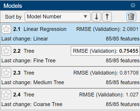
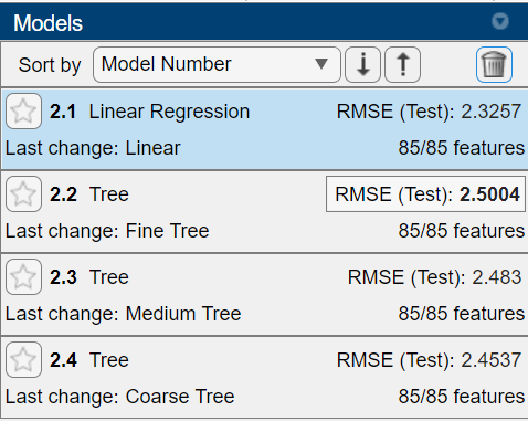
Prepare & Consider a Mannequin

There are lots of alternative ways to method this yr’s drawback, so it’s necessary to check out totally different fashions! On this tutorial, we will likely be utilizing a machine studying method to deal with the issue of climate forecasting, and for the reason that response variable ‘tmp2m’ is a quantity, we might want to create a regression mannequin. Let’s begin by opening the Regression Learner app, which can enable us to quickly prototype a number of totally different fashions.
regressionLearner
Once you first open the app, you’ll must click on on the “New Session” button within the high left nook. Set the “Knowledge Set Variable” to ‘trainingData’, and it’ll robotically choose the proper response variable. It is because it’s the final variable within the desk. Then, since it is a fairly large dataset, I alter the validation scheme to “Holdout Validation”, and set the proportion held out to fifteen. I selected these as beginning values, however you could wish to mess around with the Validation Scheme when making your personal mannequin.
After we’ve clicked “Begin Session”, the Regression Learner App interface will load.
Step 1: Begin A New Session
openRegressionLearner.gif
[Click on “New Session” > “From Workspace”, set the “Data Set Variable” to ‘trainingData’, set the “Validation Scheme” to ‘Holdout Validation’, set “percent held out” to 15, click “Start Session”]
From right here, I’m going to decide on to coach “All Fast-to-Prepare” mannequin choices, so I can see which one performs the very best out of those few. The steps for doing this are proven under. Be aware: this recording is barely sped up for the reason that coaching will take a number of seconds.
Step 2: Prepare Fashions
trainRegressionLearner.gif
[Click “All Quick-To-Train” in the MODELS section of the Toolstrip, delete the “1. Tree” model in the “Models” panel, click “Train All”, wait for all models to finish training]
I selected the “All Fast-to-Prepare” possibility in order that I might present the method, however you probably have the time, you could wish to attempt choosing “All” as a substitute of the “All Fast-to-Prepare” possibility. This gives you extra fashions to work with.
As soon as these have completed coaching, you’ll see the RMSE, or Root-Imply-Squared-Error values, proven on the left hand facet. It is a frequent error metric for regression fashions, and is what will likely be used to judge your submissions for the competitors. RMSE is calculated utilizing the next equation:


E=1n∑i=1n|Ai-Fi|2

This worth tells you ways properly the mannequin carried out on the validation information. On this case, the Nice Tree mannequin carried out the very best!
The Regression Learner app additionally allows you to import check information to see how properly the skilled fashions carry out on new information. This gives you an thought on how correct the mannequin could also be when making your closing predictions for the competitors check set. Let’s import our ‘testingData’ desk, and see how these fashions peform.
Step 3: Consider Fashions with Testing Knowledge
testRegressionLearner.gif
[Click on the “Test Data” dropdown, select “From Workspace”. In the window that opens, set “Test Data Set Variable” to ‘testingData’, then click “Import”. Click “Test All” – new RMSE values will be calculated]
This can take a couple of seconds to run, however as soon as it finishes we will see that despite the fact that the Nice Tree mannequin carried out finest on the validation information, the Linear Regression mannequin performs finest on utterly new information.
You can too use the ‘PLOT AND INTERPRET’ tab of the Regression Learner app to create visuals that present how the mannequin carried out on the check and validation units. For instance, let’s have a look at the “Predicted vs. Precise (Check)” graph for the Linear Regression mannequin:
Step 4: Plot Outcomes
testPlot.gif
[Click on the drop-down menu in the PLOT AND INTERPRET section of the Toolstrip, then select “Predicted vs. Actual (Test)”]
Since this mannequin carried out comparatively properly, the blue dots (representing the predictions) keep fairly near the road (representing the precise values). I’m proud of how properly this mannequin performs, so lets export it to the workspace so we will make predictions on different datasets!
Step 5: Export the Mannequin
[In the EXPORT section of the Toolstrip, click “Export Model” > “Export Model”. In the window that appears, click “OK”]
Now the mannequin is within the MATLAB Workspace as “trainedModel” so I can use it outdoors of the app.
To study extra about exporting fashions from the Regression Learner app, try this documentation web page!

Save and Export Predictions

Upon getting a mannequin that you’re proud of, it’s time to make predictions on new information. To point out you what this workflow seems to be like, I’m going to take away the “tmp2m” variable from my testing dataset, as a result of the competitors check set won’t have this variable.
testingData = removevars(testingData, “tmp2m”);
Now now we have a dataset that accommodates the identical variables as our coaching set besides for the response variable. To make predictions on this dataset, use predictFcn:
tmp2m = trainedModel.predictFcn(testingData);
This returns an array containing one prediction per row of the check set. To arrange these predictions for submission, we’ll must create a desk with two columns: one containing the index quantity, and one containing the prediction for that index quantity. For the reason that dataset I’m utilizing doesn’t present an index quantity, I’ll create an array with index numbers to indicate you what the ensuing desk will seem like.
index = (1:size(tmp2m))’;
outputTable = desk(index, tmp2m);
head(outputTable)
index tmp2m
_____ ______1 11.037
2 11.041
3 11.046
4 11.05
5 11.054
6 13.632
7 13.636
8 13.641
Then we will export the outcomes to an excel sheet to be learn and utilized by others!
writetable(outputTable, “datathonSubmission.csv”);
To study extra about submission and analysis for the competitors, consult with the Kaggle web page.

Experiment!

When creating any type of AI mannequin, it’s necessary to check out totally different workflows to see which one performs finest on your dataset and problem! This tutorial was solely meant to be an introduction, however there are such a lot of different selections you may make when preprocessing your information or creating your fashions. There isn’t a one algorithm that fits all issues, so put aside a while to check out totally different fashions. Listed below are some options on learn how to get began:
  • Strive different preprocessing methods, equivalent to normalizing the info or creating new variables
  • Mess around with the coaching choices obtainable within the app
  • Change the variables that you simply use to coach the mannequin
  • Strive machine and deep studying workflows
  • Change the breakdown of coaching, testing, and validaton information
In case you are coaching a deep studying community, it’s also possible to make the most of the Experiment Supervisor to coach the community underneath totally different situations and examine the outcomes!

Accomplished!

Thanks for becoming a member of me on this tutorial! We’re excited to learn how you’ll take what you may have discovered to create your personal fashions. I like to recommend wanting on the ‘Extra Sources’ part under for extra concepts on how one can enhance your fashions.
Be at liberty to succeed in out to us at studentcompetitions@mathworks.com you probably have any additional questions.

Extra Sources

  1. Overview of Supervised Studying (Video)
  2. Preprocessing Knowledge Documentation
  3. Lacking Knowledge in MATLAB
  4. Supervised Studying Workflow and Algorithms
  5. Prepare Regression Fashions in Regression Learner App
  6. Prepare Classification Fashions in Classiication Learner App
  7. 8 MATLAB Cheat Sheets for Knowledge Science
  8. MATLAB Onramp
  9. Machine Studying Onramp
  10. Deep Studying Onramp

var css=”/* Styling that’s frequent to warnings and errors is in diagnosticOutput.css */.embeddedOutputsErrorElement { min-height: 18px; max-height: 550px;} .embeddedOutputsErrorElement .diagnosticMessage-errorType { overflow: auto;} .embeddedOutputsErrorElement.inlineElement {} .embeddedOutputsErrorElement.rightPaneElement {} /* Styling that’s frequent to warnings and errors is in diagnosticOutput.css */.embeddedOutputsWarningElement { min-height: 18px; max-height: 550px;} .embeddedOutputsWarningElement .diagnosticMessage-warningType { overflow: auto;} .embeddedOutputsWarningElement.inlineElement {} .embeddedOutputsWarningElement.rightPaneElement {} /* Copyright 2015-2019 The MathWorks, Inc. *//* On this file, kinds should not scoped to rtcContainer since they might be within the Dojo Tooltip */.diagnosticMessage-wrapper { font-family: Menlo, Monaco, Consolas, “Courier New”, monospace; font-size: 12px;} .diagnosticMessage-wrapper.diagnosticMessage-warningType { colour: rgb(255,100,0);} .diagnosticMessage-wrapper.diagnosticMessage-warningType a { colour: rgb(255,100,0); text-decoration: underline;} .diagnosticMessage-wrapper.diagnosticMessage-errorType { colour: rgb(230,0,0);} .diagnosticMessage-wrapper.diagnosticMessage-errorType a { colour: rgb(230,0,0); text-decoration: underline;} .diagnosticMessage-wrapper .diagnosticMessage-messagePart,.diagnosticMessage-wrapper .diagnosticMessage-causePart { white-space: pre-wrap;} .diagnosticMessage-wrapper .diagnosticMessage-stackPart { white-space: pre;} .embeddedOutputsTextElement,.embeddedOutputsVariableStringElement { white-space: pre; word-wrap: preliminary; min-height: 18px; max-height: 550px;} .embeddedOutputsTextElement .textElement,.embeddedOutputsVariableStringElement .textElement { overflow: auto;} .textElement,.rtcDataTipElement .textElement { padding-top: 2px;} .embeddedOutputsTextElement.inlineElement,.embeddedOutputsVariableStringElement.inlineElement {} .inlineElement .textElement {} .embeddedOutputsTextElement.rightPaneElement,.embeddedOutputsVariableStringElement.rightPaneElement { min-height: 16px;} .rightPaneElement .textElement { padding-top: 2px; padding-left: 9px;}”; var head = doc.head || doc.getElementsByTagName(‘head’)[0], type = doc.createElement(‘type’); head.appendChild(type); type.sort=”textual content/css”; if (type.styleSheet){ type.styleSheet.cssText = css; } else { type.appendChild(doc.createTextNode(css)); }

RELATED ARTICLES

LEAVE A REPLY

Please enter your comment!
Please enter your name here

Most Popular

Recent Comments